Breaking New Ground: Simulating Quantum Algorithms Up to 44 Qubits on LUMI
The EuroHPC LUMI supercomputer, hosted by CSC - IT Center for Science in Kajaani, Finland, supports a wide range of world-leading research and development, from digital twins of the Earth to the formation of cosmic strings in the early universe. Now, large quantum algorithms can be efficiently simulated, pushing the frontiers for the next generation of science and discovery.
Why bother with quantum simulations when real quantum computers already exist?
Quantum computing holds the promise of revolutionizing computational modelling. Recent progress in constructing quantum computers has been rapid – already now, science that previosuly was impossible can be performed on real quantum devices. Since the first cross-border connection of an HPC system and a quantum computer within the NordIQuEst collaboration in 2022, LUMI has been at center stage for hybrid, quantum-accelerated supercomputing.
Even with real quantum computers already available, the ability to simulate quantum algorithms and circuits on a classical supercomputer is crucial. Current quantum computers belong to the so called Noisy Intermediate-Scale Quantum (NISQ) category. While valuable for scientific exploration, NISQ devices are limited by relatively high error rates and short coherence times. This implies short circuit depths, which means that current devices are limited to rather simple algorithms. On the path towards algorithms of useful complexity, simulating quantum algorithms using classical supercomputers provides a crucial tool for several reasons:
-
Validation and Verification: Classical simulations help develop, validate, and verify quantum algorithms before they are run on actual quantum hardware. This ensures that the algorithms work as intended and helps identify potential errors.
-
Understanding Quantum Systems: These simulations provide insights into the behavior of quantum circuits, which is essential for developing more efficient quantum algorithms which will help pave a path towards prioritizing the improvements that will be made to future quantum hardware.
-
Debugging of quantum software: In contrast to physical quantum computers, simulators provide the opportunity to, for example, follow the evolution of quantum states throughout the simulation. Physical qubits do not allow probing the state of a qubit during the calculation.
-
Development of Hybrid Systems: Classical simulations are instrumental in the development phases of hybrid quantum-classical systems, where both types of computing are used together to solve complex problems.
Practical simulation limits
There are several different approaches to simulating quantum algorithms with classical computers. They can, arguably, be divided into two main classes: tensor network simulations and full state-vector simulations. While tensor network simulations have been used to simulate algorithms of thousands of qubits, they come with an inherent limitation: they are only suitable for quantum algorithms with a rather low degree of entanglement between the qubits. Entanglement, the “spooky action at a distance” as Einstein infamously called it, is a pre-requisite for many of the use cases where quantum computing is expected to provide tangible advantage. After all, if a quantum algorithm can be efficiently simulated on a classical computer, there is less need for a quantum computer to begin with.
For exploring algorithms utilising higher levels of entanglement, a “Schrödinger-style” full state-vector simulation becomes necessary. This type of simulation is generally much more resource intensive but offers the advantage of detailed inspection of how the quantum states change and develop during the execution of the algorithm. This is where the need for supercomputers enters, and the topic of this blog.
Simulating quantum circuits is highly resource consuming, especially when the number of qubits grow beyond approximately thirty. Here, we report a simulation of up to 44 qubits using the full state-vector method of qiskit-aer [1] using 4096 GPGPUs (General Purpose Graphics Processing Units) across 1024 nodes. For a simulation of this size, powerful supercomputing resources are needed, as the required memory just for storing the quantum state information of the qubits grows exponentially with qubit count:
\[\text{Memory} = \text{precision} \times 2^n\]For n = 44 qubits with 16-byte precision:
\[16 \times 2^{44} = 256 \, \text{TB}\]High end laptops / desktops are typically available with memory configurations of around 64-256 GB. This allows for a state-vector simulation of 31-33 qubits only. A single node in the LUMI standard-g partition has approximately 480 GB of useable memory for HPC workloads. This increases the simulation capacity beyond what a typical personal computer can achieve, but is still insufficient for a state-vector simulation of 44 qubits.
The Table below illustrates the amount of memory required for running state-vector simulation data using double precision. Every time the number of qubits is increased by one, the qubit memory requirements for a state-vector simulation is doubled. To simulate more than 34 qubits requires breaking beyond the limits of the local memory space within a single node – we need to parallelize across the nodes of the supercomputer.
| # of Qubits | Memory requirements |
|---|---|
| 32 | 64 GB |
| 33 | 128 GB |
| 34 | 256 GB |
| 36 | 1024 GB |
| 38 | 4 TB |
| 40 | 16 TB |
| 42 | 64 TB |
| 44 | 256 TB |
Hardware Specifications for a single node
This table shows the hardware resources available [3] on a single compute node in the LUMI standard-g partition.
| LUMI single GPU accelerated node | Specifications |
|---|---|
| LUMI Partition | standard-g |
| Model of node | HPE Cray EX |
| CPU Model | AMD EPYC Trento |
| # of CPU sockets | 1 |
| # of CPU cores | 64 |
| GPU Model | AMD Instinct MI250X GPU |
| AMD Rocm version | 6.1.2 |
| # of GPUs (GCDs) | 8 |
| Amount of memory per GPU | 64 GB |
| Amount of Useable system memory | 480 GB |
| Network | HPE Cray Slingshot-11 200 Gbps NIC using Dragonfly topology |
Surpassing simulation limits of a single node
To overcome the memory limitations imposed by large qubit counts requires utilizing the distributed memory spaces across many nodes by leveraging MPI (Message Passing Interface). MPI is a portable message-passing standard designed to function on parallel computing architectures, and allows for utilizing both the CPUs/GPUs and their distributed memory across many compute nodes.
Parallelizing a simulation across multiple nodes
Using MPI we can aggregate the system memory of many nodes for our simulation. Below is a table that shows the memory requirements of storing the state-vector information of our quantum state as well as the amount of useable system memory distributed across the number of nodes that we use for simulation of n qubits.
| n # of Qubits | Memory requirements | Number of nodes | Available system memory |
|---|---|---|---|
| 34 | 256 GB | 1 | 480 GB |
| 35 | 512 GB | 2 | 960 GB |
| 36 | 2048 GB | 4 | 1920 GB |
| 38 | 4 TB | 16 | 7.5 TB |
| 40 | 16 TB | 64 | 30 TB |
| 42 | 64 TB | 256 | 120 TB |
| 44 | 256 TB | 1024 | 480 TB |
Using GPUs to accelerate Quantum simulations
Now that system memory requirements needed for simply storing the state-vector information of our qubits have been worked out, we can pivot to speeding up our simulation execution times using GPU acceleration and cache blocking techniques. Let’s first shed some light on why GPU accelerated hardware speeds up the simulations.
The type of calculations used in state-vector simulations of quantum circuits makes GPUs a natural choice for acceleration due to several key factors:
-
Linear Algebra Operations
State-vector simulations rely heavily on linear algebra operations like matrix multiplications and vector additions. These operations are inherently parallel, meaning they can be divided into smaller tasks that can be executed simultaneously. GPUs are designed for this type of parallel processing, making them more efficient as an accelerator for these computations. -
Massive Parallelism
GPUs have a large number of cores (thousands of threads), which allows them to handle many operations at the same time. Since the workload of state-vector quantum circuit simulation is massively parallel, using GPUs is a good choice for accelerating such tasks. -
High Memory Bandwidth
Simulations of quantum states can involve large datasets, which can put a strain on memory access. GPUs typically have high-bandwidth memory (such as HBM2e), which allows for faster data retrieval and minimizes delays caused by memory bottlenecks, especially as the number of qubits increases. -
Efficient Floating-Point Operations
Quantum simulations often require high-precision floating-point calculations, such as those involving complex numbers. GPUs are capable of efficiently performing both single and double-precision floating-point operations, which are needed for the precision required in these simulations. -
Support for Optimized Libraries
GPUs are supported by libraries that are specifically optimized for accelerating tasks like matrix operations and Fourier transforms, which are common in quantum simulation domain. These libraries are tailored to GPU architecture, improving the performance of these operations. -
Scalability Across HPC Nodes
As quantum simulations grow in complexity with more qubits, they often need to be distributed across multiple computing nodes. GPUs are well-suited for this kind of parallel computation across many nodes, allowing simulations to scale to larger systems than what would be feasible with a single machine. -
Energy Efficiency and Cost-Effectiveness
Compared to CPU-based systems, GPUs are generally more energy-efficient for the kind of parallel processing needed in large-scale simulations. This can reduce the operational cost for running simulations of large quantum circuits.
Using Cache blocking with GPUs to accelerate Quantum Simulations
To speed up simulations, we employed a technique called cache blocking, in which parts of quantum circuit (chunks) are simulated parallel in distributed memory spaces (caches). An important factor to condsider when using cache blocking is the data transfer between caches. When chunks that are far apart in memory need to interact, data has to be transferred over the network between those memory locations. This data transfer (or “data exchange”) between compute nodes is relatively slow and becomes a bottleneck when utilizing large amount of resources.
By strategically rerouting quantum operations using simulated noiseless SWAP gates, frequently interacting qubits are grouped together in memory on a single node; thereby reducing the need for slow data transfers between different distributed memory spaces spread out across the nodes of the supercomputer. This optimization technique draws inspiration from classical cache blocking methods and is implemented within Qiskit Aer to improve its performance, especially when dealing with large, complex quantum circuits. Also, by utilizing additional memory spaces for buffering, the data exchange between chunks can be decreased, making the simulation more efficient. [4] [5].
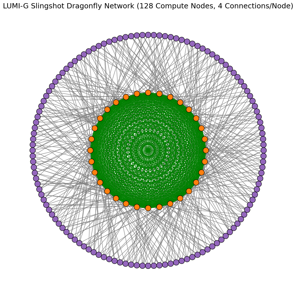
Example connectivity graphs showing network traffic between LUMI-G nodes
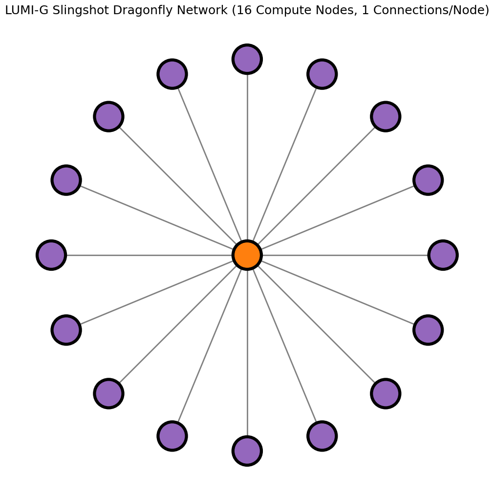
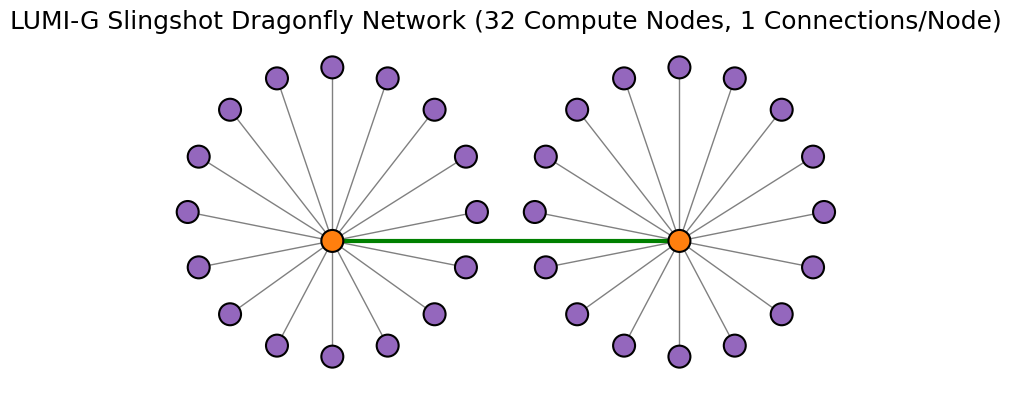
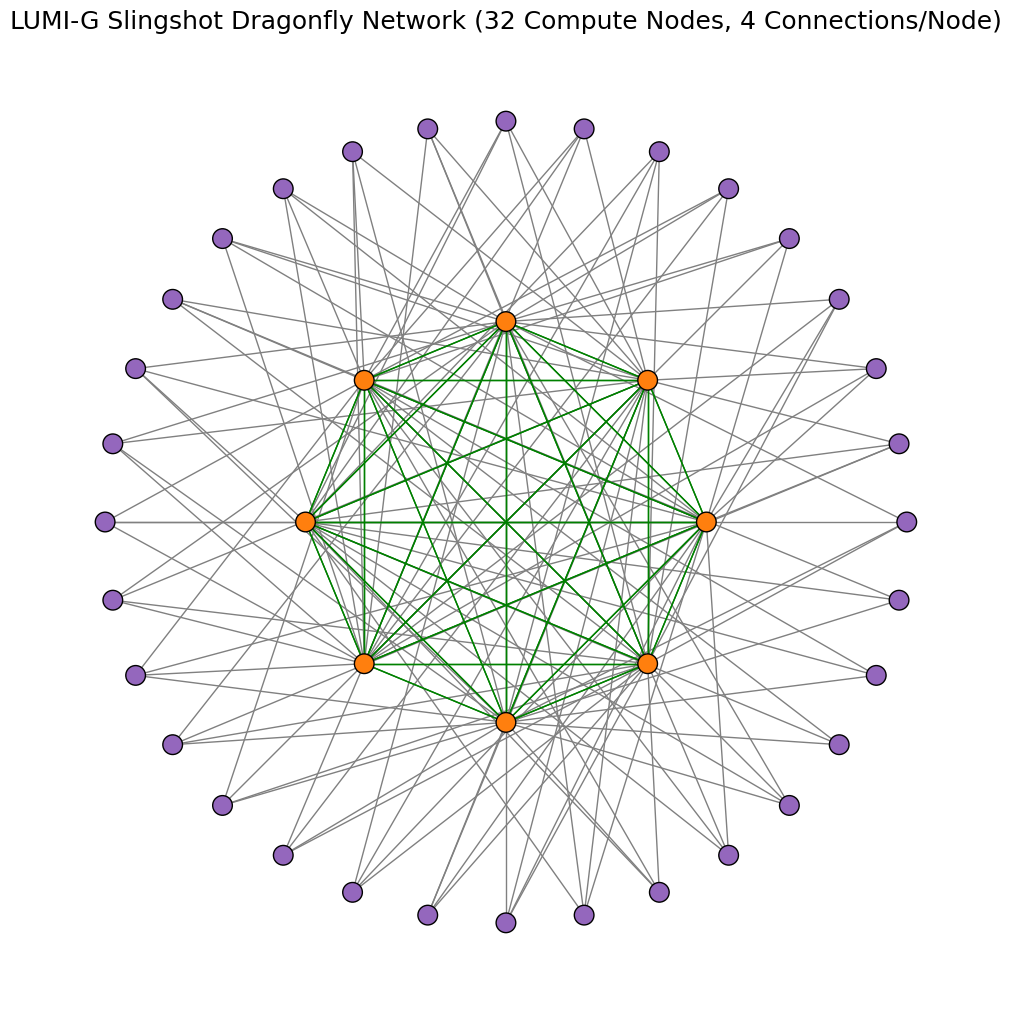
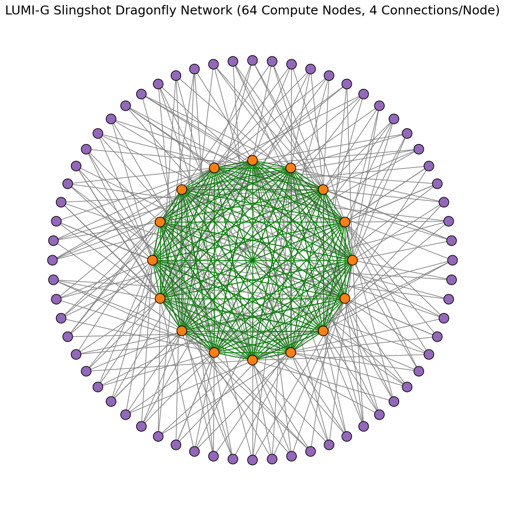
In the LUMI-G partition, nodes are connected to each other by switches. Each node has 4 network connections, and single switch can have maximum of 16 nodes connected. In image below, the compute nodes are marked as purple dots and slingshot switches as orange dots. The gray lines show network connectivity (1 hop) between a compute node and a switch. The green lines show the network connectivity between switches (1 hop). The maximum hops that any network traffic can take between nodes on the LUMI-G slingshot network are 3.
The example graphs below demonstrate the minimum possible data exchange paths for 2 different simulations that may take place between 16 nodes (38 qubits) and 32 nodes (39 qubits) over the Cray/HPE Slingshot network. This demonstrates the utility of trying to use the local memory space of a nodes before accessing distributed memory spaces. Localized computations take place within the nodes before having to transfer data across the network, a requirement for data exhange between caches. For example, when using 16 nodes connected by single switch, any data exhange between nodes goes through a maximum of 2 hops.
“Necessity is the mother of invention” - Building a container for scaling simulations
When our users inquired about running multinode simulations with Qiskit, we took the task of building a Qiskit Aer singularity container with support for the AMD ROCm GPUs using Native HPE Cray MPI as suggested by the LUMI documentation.
Multiple container build iterations took place before arriving at the latest version of qiskit/qiskit-aer. The biggest performance improvements in the qiskit-aer container comes from the usage of the same Native HPE Cray MPI software that is built on the node.
In order to build a performant container, some tradeoffs were made.
Pros:
- The container exhibits a drastic performance gain.
- New containers are easy to maintain as each container in the build process manages different aspects of the software stack.
Cons:
- Lack of portability.
- Built specifically for LUMI nodes that use HPE Cray MPI.
- Increased complexity in curating container build scripts and definitions specific to LUMI.
- A new container must be rebuilt after a major system update on LUMI.
These drawbacks are easily outweighed by the substantial performance increase in the simulations – a drastic (8x) speedup, as seen in the test outputs below.
Example Simulation using a container built using ABI Compliant MPICH
Singularity Container   : /<ProjectDIR>/ABI-compliant-MPICH_qiskit_csc.sif
Simulation Method       : statevector
# of Qubits             : 36
# of Blocking Qubits    : 30
Circuit Depth           : 10
NODES                   : 8
Tasks Per Node          : 8
CPUS PER TASK           : 7
GPU LIST                : 0,1,2,3,4,5,6,7
Simulation Execution time: 130.7357989
Example Simulation using a container built using HPE Cray MPI
Notice the Speedup in simulation time.
Singularity Container   : /<ProjectDIR>/HPE-Cray-MPI_qiskit_csc.sif
Simulation Method       : statevector
# of Qubits             : 36
# of Blocking Qubits    : 30
Circuit Depth           : 10
NODES                   : 8
Tasks Per Node          : 8
CPUS PER TASK           : 7
GPU LIST                : 0,1,2,3,4,5,6,7
Simulation Execution time: 16.12554312
These results clearly justify the additional effort.
Container information used in tests
OS:
Bootstrap: docker
From: opensuse/leap:15.5
GPU :
%applabels rocm

VERSION       6.0.3
PYTHON
%applabels python

VERSION       3.11.10
SIMULATION SOFTWARE:
qiskit==1.3.2
qiskit-aer-gpu==0.16.0
qiskit-algorithms==0.3.1
qiskit-dynamics==0.5.1
qiskit-experiments==0.8.1
qiskit-finance==0.4.1
qiskit-ibm-experiment==0.4.8
qiskit-machine-learning==0.8.2
qiskit-nature==0.7.2
qiskit-optimization==0.6.1
qiskit_qasm3_import==0.5.1
Scaling Experiments: Performance Evaluation of Qubit Simulations
It is important to define resource allocations that offer a balance of performance and efficient utilization of LUMI’s compute and memory resources. To provide general examples of algorithm execution times, we ran a series of Quantum Volume (QV) simulations of various depth to systematically evaluate the performance of state-vector simulator on LUMI. The QV algorithm and the types of tests are based on similar tests presented in previous research [6] [7] [8]. A battery of three tests were conducted:
- Single Node Performance
- Strong Scaling Analysis
- Weak Scaling Analysis
Each of these tests provide insights into the computational feasibility, efficiency, and limitations of qubit simulations using the standard-g GPU accelerated partition of LUMI.
1. Single Node Performance
Objective:
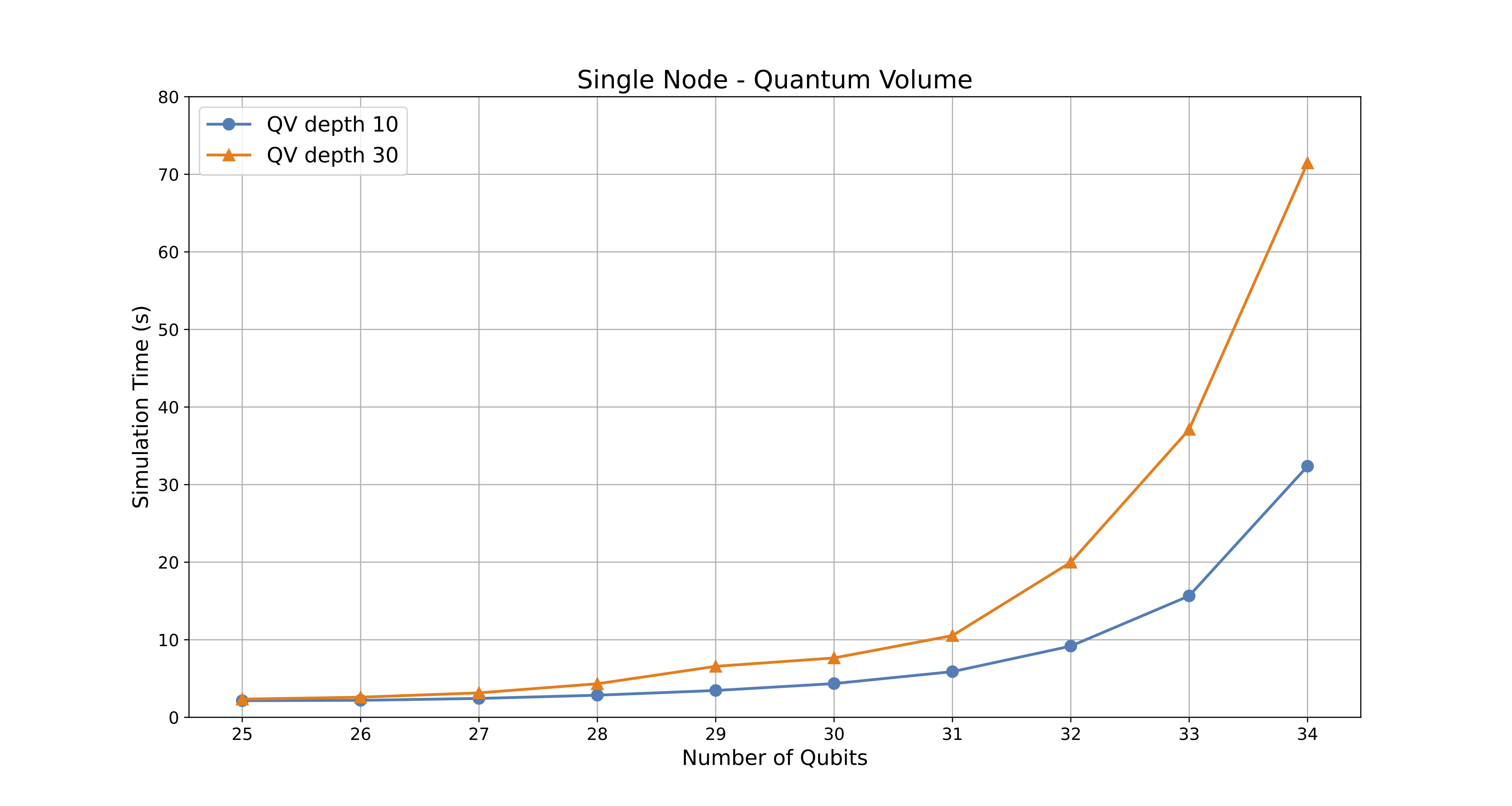
Assess the performance limits of simulating quantum circuits on a single LUMI standard-g node, determining the maximum number of qubits that can be handled before encountering memory or performance bottlenecks. The execution time of two tests, corresponding to circuit depths of 10 and 30, is analyzed over a qubit range of 25 to 34.
Algorithm & Justification:
-
Methodology:
The experiment was conducted on a single node with 8 GPUs allocated to a single task. The number of qubits was gradually increased from 25 to 34, and execution times were recorded for circuit depths of 10 and 30. This setup isolates node-level performance, eliminating multi-node communication effects, allowing for a clear analysis of computational scalability within a single LUMI standard-g node. -
Justification:
Understanding single-node performance is crucial for defining the baseline computational capacity of the system. This experiment provides insight into how execution time scales with an increasing number of qubits and highlights the limits of single-node simulations before requiring distributed computation.
Results & Discussion:
-
Performance Trends:
The execution time increases with the number of qubits, with a noticeable acceleration as the qubit count approaches 34. The simulation time scales linearly with circuit depth, as expected. However, for a fixed circuit depth, the time increases non-linearly with qubit count, as expected from the increased computational complexity. -
Efficiency Losses:
Since this is a single-node experiment, the losses are due to intra-node computational challenges and not inter-node communication.-
Memory Bottlenecks:
The rapid increase in execution time for higher qubit counts (e.g., 32–34 qubits) indicates that memory bandwidth and GPU utilization limits start becoming significant, even if there is sufficient memory to carry out the calculation. -
GPU Utilization Saturation:
The GPUs reach saturation as the problem size grows, leading to diminishing performance gains from hardware parallelism. This can be seen in the GPU statistics in the experimental data presented below. -
Cache and Data Transfer Overhead:
Simulating highly entangled quantum states using requires incresing the amount of caches, leading to more frequent data movement between local and distributed memory hierarchies, contributing to increasing execution time. Additionally, the higher qubit counts require exponential increases in memory which is distributed across a greater number of nodes. As the amount of nodes increases, so does the complexity of data exchanges across the network of nodes. See Figures 1 and 2. -
Algorithmic Complexity:
The simulation’s inherent exponential growth in state space representation contributes to an unavoidable increase in runtime.
-
Quantum Volume - Single Node execution time results table
| Qubits | Blocking Qubits | Allocated Nodes | Allocated GPUs | Tasks Per Node | Circuit Execution Time (Depth 10) - Seconds | Circuit Execution Time (Depth 30) - Seconds |
|---|---|---|---|---|---|---|
| 25 | 0 | 1 | 8 | 1 | 2.147 | 2.349 |
| 26 | 0 | 1 | 8 | 1 | 2.193 | 2.598 |
| 27 | 0 | 1 | 8 | 1 | 2.436 | 3.156 |
| 28 | 0 | 1 | 8 | 1 | 2.854 | 4.329 |
| 29 | 0 | 1 | 8 | 1 | 3.463 | 6.577 |
| 30 | 29 | 1 | 8 | 1 | 4.352 | 7.656 |
| 31 | 29 | 1 | 8 | 1 | 5.890 | 10.536 |
| 32 | 29 | 1 | 8 | 1 | 9.183 | 19.993 |
| 33 | 29 | 1 | 8 | 1 | 15.656 | 37.115 |
| 34 | 29 | 1 | 8 | 1 | 32.371 | 71.462 |
GPU Statistics for a 32 Qubit Simulation on a single LUMI-G node
notice the GPU VRAM usage (38%), and not all GPUs are at a constant 100% utilization
> srun --interactive --pty --jobid=<SLURM_JOBID> rocm-smi


======================================== ROCm System Management Interface ========================================
================================================== Concise Info ==================================================
Device  [Model : Revision]    Temp    Power   Partitions      SCLK     MCLK     Fan  Perf    PwrCap  VRAM%  GPU%
        Name (20 chars)       (Edge)  (Avg)   (Mem, Compute)
==================================================================================================================
0       [0x0b0c : 0x00]       55.0°C  292.0W  N/A, N/A        1425Mhz  1600Mhz  0%   manual  500.0W   38%   100%
        AMD INSTINCT MI200 (
1       [0x0b0c : 0x00]       51.0°C  N/A     N/A, N/A        1425Mhz  1600Mhz  0%   manual  0.0W     38%   100%
        AMD INSTINCT MI200 (
2       [0x0b0c : 0x00]       44.0°C  277.0W  N/A, N/A        1650Mhz  1600Mhz  0%   manual  500.0W   38%   100%
        AMD INSTINCT MI200 (
3       [0x0b0c : 0x00]       48.0°C  N/A     N/A, N/A        1650Mhz  1600Mhz  0%   manual  0.0W     38%   0%
        AMD INSTINCT MI200 (
4       [0x0b0c : 0x00]       49.0°C  286.0W  N/A, N/A        1390Mhz  1600Mhz  0%   manual  500.0W   38%   100%
        AMD INSTINCT MI200 (
5       [0x0b0c : 0x00]       53.0°C  N/A     N/A, N/A        800Mhz   1600Mhz  0%   manual  0.0W     38%   2%
        AMD INSTINCT MI200 (
6       [0x0b0c : 0x00]       51.0°C  275.0W  N/A, N/A        1425Mhz  1600Mhz  0%   manual  500.0W   38%   100%
        AMD INSTINCT MI200 (
7       [0x0b0c : 0x00]       52.0°C  N/A     N/A, N/A        1425Mhz  1600Mhz  0%   manual  0.0W     38%   100%
        AMD INSTINCT MI200 (
==================================================================================================================
============================================== End of ROCm SMI Log ===============================================
GPU Statistics for a 34 Qubit Simulation on a single LUMI-G node
notice the increased GPU VRAM usage (63%) and all GPUs at 100% utilization
> srun --interactive --pty --jobid=<SLURM_JOBID> rocm-smi


======================================== ROCm System Management Interface ========================================
================================================== Concise Info ==================================================
Device  [Model : Revision]    Temp    Power   Partitions      SCLK     MCLK     Fan  Perf    PwrCap  VRAM%  GPU%
        Name (20 chars)       (Edge)  (Avg)   (Mem, Compute)
==================================================================================================================
0       [0x0b0c : 0x00]       50.0°C  302.0W  N/A, N/A        1515Mhz  1600Mhz  0%   manual  500.0W   63%   100%
        AMD INSTINCT MI200 (
1       [0x0b0c : 0x00]       59.0°C  N/A     N/A, N/A        1515Mhz  1600Mhz  0%   manual  0.0W     63%   100%
        AMD INSTINCT MI200 (
2       [0x0b0c : 0x00]       52.0°C  287.0W  N/A, N/A        1540Mhz  1600Mhz  0%   manual  500.0W   63%   100%
        AMD INSTINCT MI200 (
3       [0x0b0c : 0x00]       50.0°C  N/A     N/A, N/A        1535Mhz  1600Mhz  0%   manual  0.0W     63%   100%
        AMD INSTINCT MI200 (
4       [0x0b0c : 0x00]       45.0°C  295.0W  N/A, N/A        1500Mhz  1600Mhz  0%   manual  500.0W   63%   100%
        AMD INSTINCT MI200 (
5       [0x0b0c : 0x00]       48.0°C  N/A     N/A, N/A        1500Mhz  1600Mhz  0%   manual  0.0W     63%   100%
        AMD INSTINCT MI200 (
6       [0x0b0c : 0x00]       43.0°C  285.0W  N/A, N/A        1525Mhz  1600Mhz  0%   manual  500.0W   63%   100%
        AMD INSTINCT MI200 (
7       [0x0b0c : 0x00]       52.0°C  N/A     N/A, N/A        1515Mhz  1600Mhz  0%   manual  0.0W     63%   100%
        AMD INSTINCT MI200 (
==================================================================================================================
============================================== End of ROCm SMI Log ===============================================
Quantum Volume - Single Node execution time results - chart
2. Strong Scaling Analysis
Objective:
Evaluate how simulation time decreases as the number of compute nodes increases for a fixed number of qubits (34). The analysis explores six different node allocations (1, 2, 4, 8, 16, 32 nodes) across four circuit depths (10, 30, 100, 300), highlighting the impact of parallelization on execution time.
Algorithm & Justification:
-
Methodology:
The experiment was conducted with a fixed qubit count of 34, progressively increasing the allocated compute nodes from 1 to 32 while keeping 8 GPUs per node. Each node was assigned 8 tasks, leading to a total of 256 MPI ranks at the highest allocation level. Execution times were recorded for circuit depths 10, 30, 100, and 300 to assess scaling behavior across shallow and deep circuits. -
Justification:
Quantum circuit simulations can be accelerated by increasing computational resources, enabling faster feedback for quantum algorithm designers. This study quantifies the efficiency of distributing workloads across more nodes, balancing speedup versus resource use. However, excessive resource allocation can lead to diminishing returns or even execution failures due to exceeding parallelization limits.
Results & Discussion:
-
Performance Trends:
Increasing the number of nodes reduces execution time, particularly for deeper circuits. For this specific example, the largest speedup is observed between 1 and 8 nodes. Although the simulation execution time does scales well up to 32 nodes, the performance improvements begin to diminish beyond 8 nodes. -
Efficiency Losses:
While increasing resources enhances performance, efficiency losses emerge at higher allocations due to:-
Communication Overhead:
MPI-based communication increases as more nodes are used, contributing to diminishing returns at 16+ nodes. -
Synchronization Delays:
Larger task distributions require more frequent synchronization, particularly for deep circuits, impacting performance gains. -
Load Balancing Challenges:
At higher node counts, work imbalance can arise, as certain tasks may complete before others, leading to idle resources. -
Parallelization Limits:
The maximum effective MPI ranks that can be used for a given qubit count is constrained by the simulation’s computational structure. Over-allocation of nodes can result in execution failures, as seen when exceeding the optimal distribution.
-
-
Scaling Efficiency:
Strong scaling tests for quantum volume circuit with 34 qubits run very efficiently up to 16 nodes, with diminishing efficiency beyond 32 nodes. While increasing node allocations can accelerate simulations, optimal resource allocation depends on circuit depth and computational workload. Generally, doubling the number of nodes does not always halve the execution time.
Calculating Max Nodes for our tests
Before running the tests, some awareness about the test parameteres that can and can not be used is needed, based on some initial assumptions and quick math. To obtain an estimate of the maximum number of nodes for error-free execution of a job, the formula below provides some guidance.
\[\begin{aligned} \text{mem[statevec]} &\quad = \quad \text{precision} \times 2^n \\ \text{mem[cache]} &\quad = \quad \text{precision} \times 2^{c} \\ \end{aligned}\], where n is number of qubits and c is the number of cache blocking qubits
\[\begin{aligned} \text{Max MPI Ranks} &\quad = \quad \frac{\text{mem[statevec]}}{\text{mem[cache]}} \\ %&\quad = \quad \frac{\text{precision} \times 2^n}{\text{precision} \times 2^{c}} \\ &\quad = \quad 2^{n - c} \\ \\ \text{Max Nodes} &\quad = \quad \frac{\text{Max MPI Ranks}}{\text{Tasks Per Node}} \end{aligned}\]Using the above formulas to calculate Max Nodes with respect to our chosen value for n qubits and c cache-blocking qubits we can compare the results of the formula to the error message
Example Error
mpi_test_34_qubits_29_blocking_8_GPU_8_task_8_node_depth_10.e9525960

Simulation failed and returned the following error message:
ERROR:  [Experiment 0] cache blocking : blocking_qubits is too large to parallelize with 64 processes
Simulation failed and returned the following error message:
Using the Following allocation resources
mpi_test_34_qubits_29_blocking_8_GPU_8_task_8_node_depth_10.o9525960

Singularity Container   : /appl/local/quantum/qiskit/qiskit_1.3.2_csc.sif
Simulation Method       : statevector
# of Qubits             : 34
# of Blocking Qubits    : 29
Circuit Depth           : 10
SLURM JOB NAME          : mpi_test_34_qubits_29_blocking_8_GPU_8_task_8_nodes_depth_10
SLURM JOB ID            : 9525960
NODES                   : 8
NODE LIST               : nid[005322-005323,005356-005357,005423,007447-007449]
Tasks Per Node          : 8
CPUS PER TASK           : 7
GPUS PER NODE           : 8
GPU LIST                : 0,1,2,3,4,5,6,7
Step 1: Express Max MPI Ranks in terms of Max Nodes: Calculation of Max Nodes for given number of total qubits and cache-blocking qubits. We use parameters from the above error message
\[\begin{aligned} n &\quad = \quad \text{34} \\ c &\quad = \quad \text{29} \\ \\ \text{Max MPI ranks} &\quad = \quad 2^{n - c} \\ %\\ %\text{Max MPI Ranks} &\quad = \quad 2^{5} \\ &\quad = \quad 32 \\ \\ \text{Max Nodes} &\quad = \quad \frac{\text{Max MPI Ranks}}{\text{Tasks Per Node}} \\ %&\quad = \quad \frac{\text{32}}{\text{8}} \\ &\quad = \quad \text{4} \\ \\ \end{aligned}\]The above experiment failed due to the amount of allocated nodes (Max Nodes) being 8 (64 parallel processes) rather than 4 (32 parallel processes). There were not enough MPI ranks (distributed processess) to spread out across the amount of nodes that were requested in the resource allocation. The 64 processes are double the amount of Max MPI Ranks (32) that would be spawned based on the size of the cache-blocking qubits used for a simulation of n qubits. Now if we work backwards knowing that we want to run an experiment on 8 nodes, we can calculate the size of c cache-blocking qubits in with respect to the number of n qubits and Tasks Per Node as can be observed in the example below. Notice that if we decrease the cache-blocking qubits from 29 to 28 we are able to generate enough parallel processes (64) to be distributed across 8 nodes:
Step 2: Solve for cache-blocking qubits: Calculation for suitable number of cache-blocking qubits for given number of nodes and qubits
\[\begin{aligned} \\ n &\quad = \quad \text{34} \\ \text{Max Nodes} &\quad = \quad \text{8} \\ \text{Tasks per Node} &\quad = \quad \text{8} \\ \\ \text{Max MPI Ranks} &\quad = \quad (\text{Max Nodes} \times \\ &\quad\quad\quad\text{Tasks Per Node}) \\ &\quad = \quad \text{64} \\ \\ \\ \text{Max MPI Ranks} &\quad = \quad 2^{n-c} \\ \\ \Rightarrow c &\quad = \quad n - \log_2(\text{Max MPI} \\ &\quad\quad\quad\quad\quad\quad\quad \text{Ranks}) \\ &\quad = \quad 34 - \log_2 (\text{64}) \\ &\quad = \quad 28 \end{aligned}\]Equipped with the tools needed to estimate the resource needs before submitting jobs, we proceed with the Strong Scaling tests.
Quantum Volume - Strong Scaling execution time results table
| # of Qubits | Blocking Qubits | Allocated Nodes | Allocated GPUs | Tasks Per Node | Total Tasks (MPI Ranks) | Circuit Execution Time (Depth 10) - seconds | Circuit Execution Time (Depth 30) - seconds | Circuit Execution Time (Depth 100) - seconds | Circuit Execution Time (Depth 300) - seconds |
|---|---|---|---|---|---|---|---|---|---|
| 34 | 26 | 1 | 8 | 8 | 8 | 17.704 | 53.813 | 157.277 | 451.620 |
| 34 | 26 | 2 | 8 | 8 | 16 | 14.196 | 40.388 | 118.691 | 338.842 |
| 34 | 26 | 4 | 8 | 8 | 32 | 9.117 | 23.768 | 73.050 | 200.675 |
| 34 | 26 | 8 | 8 | 8 | 64 | 5.721 | 13.236 | 41.134 | 113.088 |
| 34 | 26 | 16 | 8 | 8 | 128 | 3.536 | 7.980 | 22.074 | 59.613 |
| 34 | 26 | 32 | 8 | 8 | 256 | 2.645 | 5.232 | 13.063 | 35.655 |
Quantum Volume - Strong Scaling execution time results - chart
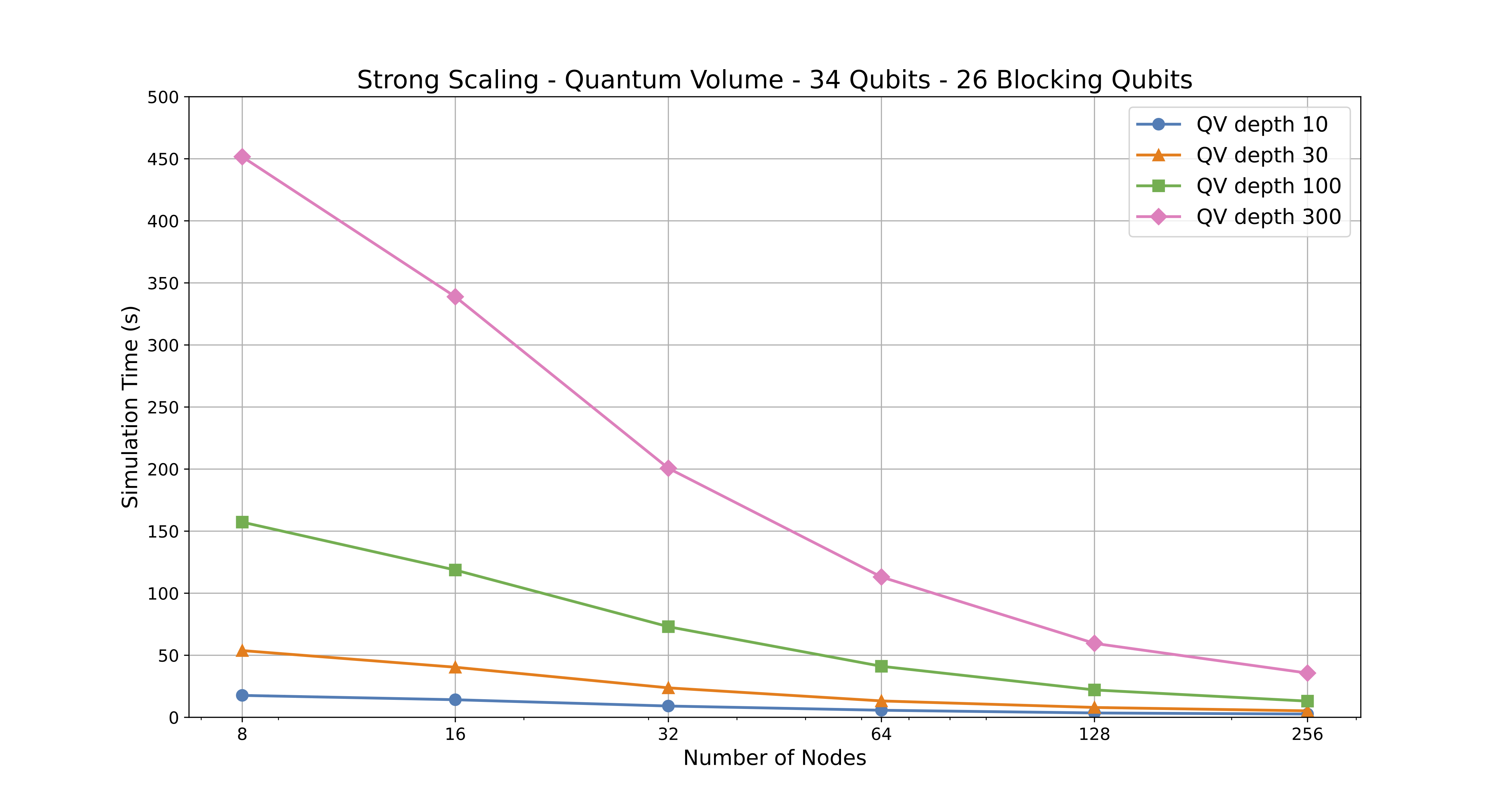
Figure 4: Chart displaying the execution time of Quantum Volume depth 10, 30, 100, and 300 on a range of nodes.
Figuring out the optimal size for cache-blocking qubits for the Strong Scaling tests
You may have noticed that for the strong scaling experiment, a cache blocking qubit size (c) of 26 was chosen. This number was chosen so that there would be 6 datapoints for each Strong Scaling QV experiment (depth 10, 30, 100, and 300). To do this we chose the following amount of nodes 1, 2, 4, 8, 16, and 32.
Assuming that we keep the following other resource allocations static: Tasks Per Node, GPUs per node, we can figure out the optimal value for c based on the amount of n qubits in our simulation and the max amount of nodes that we wish to allocate for a simulation.
Step 1: Express Max MPI Ranks in terms of Max Nodes: Similarly as in single node example, the number of MPI ranks can be expressed in terms of total number of qubits $n$ and number of cache-blocking qubits $c$
\[\text{Max MPI ranks} = 2^{n - c} \\\]Step 2: Solve for cache-blocking qubits Again repeating the calculation from single node example, we get proper amount of cache-blocking qubits by solving $c$ from above equation. Setting Max Nodes to Nodes(32), while keeping the number of qubits (34) and Task per node(8), and Max MPI Ranks(64) the same
\[\begin{aligned} n &\quad = \quad 34 \\ \text{Max Nodes} &\quad = \quad 32 \\ \text{Tasks per Node} &\quad = \quad 8 \\ \\ \text{Max MPI Ranks} &\quad = \quad (\text{Max Nodes} \times \\ &\quad\quad\quad\text{Tasks Per Node}) \\ &\quad = \quad 256 \\ \\ \Rightarrow c &\quad = \quad n - \log_2(\text{Max MPI} \\ &\quad\quad\quad\quad\quad\quad\quad \text{Ranks}) \\ &\quad = \quad 34 - \log_2 (256) \\ &\quad = \quad 26 \end{aligned}\]3. Weak Scaling Analysis
Objective: To evaluate performance when both the number of qubits and compute nodes increase proportionally, ensuring memory per node remains constant.
Algorithm & Justification:
-
Methodology: The weak scaling analysis is performed by increasing the number of qubits simulated while simultaneously increasing the number of compute nodes in order to accomodate the memory requirements of the qubits. The key idea is to keep the computational load per node approximately constant. This is achieved by fixing the number of blocking qubits c (29 in this case). Each node is assigned a subset of the total quantum system to simulate. As the total number of qubits grows, the number of nodes is increased to handle the larger simulation’s memory requirements, but each node’s share of the work remains roughly the same. The number of MPI Tasks Per Node is also held constant at 8. This means that the total number of MPI ranks (parallel processes) increases linearly with the number of nodes.
-
Justification: Weak scaling is appropriate for this problem because state-vector simulations of quantum systems are highly memory-intensive. The memory required to store the quantum state grows exponentially with the number of qubits. By using weak scaling, we can investigate how the simulation performs as we scale up to larger quantum systems, under the constraint of a fixed memory footprint per compute node. This mirrors a common scenario in high-performance computing, where you want to solve larger problems by using more resources, without exceeding the memory capacity of individual nodes. It helps to understand the parallel efficiency of the simulation tooling.
Results & Discussion:
-
Performance Trends: The table shows that as the number of qubits (and nodes) increases, the execution time for both circuit depths (10 and 30) also increases. However, the rate of increase is not perfectly linear. Ideally, in perfect weak scaling, the execution time would remain constant as the problem size and the number of nodes increase proportionally. The observed increase in execution time indicates that there is some overhead associated with the parallel computation.
-
Efficiency Losses: The deviation from ideal linear scaling represents efficiency losses. These losses are due to several factors:
-
Communication Overhead: As the number of nodes increases, the amount of communication between nodes also increases. This communication (e.g., exchanging quantum state information) takes time and becomes a bottleneck.
-
Synchronization Overhead: The parallel processes running on different nodes need to synchronize their operations. This synchronization also introduces overhead, as nodes may have to wait for each other.
-
Load Imbalance: Although the problem is divided equally among nodes, there might be slight variations in the computational load on different nodes. Some nodes might finish their assigned work slightly earlier than others, leading to idle time and reduced efficiency.
-
Increased complexity: As the number of qubits increases, the complexity of the quantum circuits might also increase, leading to a non-linear increase in computation time.
-
-
Scaling with Problem Size: The simulation scales to larger problem sizes by utilizing more compute nodes. The memory requirements per node remain constant (as designed in the weak scaling approach). However, the execution time increases with the problem size. This shows that while the simulation can handle larger quantum systems, the efficiency of the parallel computation decreases as the number of nodes increases. The scaling is sub-optimal, but still allows for solving larger problems. The key takeaway is that the overhead of distributed computing becomes more significant as the scale of the simulation grows.
Quantum Volume - Weak Scaling - network complexity scales with allocated resources (nodes)
Quantum Volume - Weak Scaling execution time result tables
| Qubits | Blocking Qubits | Number of Nodes | Tasks Per Node | Total Tasks (MPI Ranks) | Minimum Memory Requirements (GB) | Total Usable Memory Across Nodes (GB) | Circuit Execution Time (Depth 10) - seconds | Circuit Execution Time (Depth 30) - seconds |
|---|---|---|---|---|---|---|---|---|
| 34 | 29 | 1 | 8 | 8 | 256 GB | 480 GB | 17.723 | 47.683 |
| 35 | 29 | 2 | 8 | 16 | 512 GB | 960 GB | 28.355 | 63.231 |
| 36 | 29 | 4 | 8 | 32 | 1024 GB | 1920 GB | 31.728 | 88.154 |
| 37 | 29 | 8 | 8 | 64 | 2 TB | 4 TB | 32.785 | 94.958 |
| 38 | 29 | 16 | 8 | 128 | 4 TB | 8 TB | 39.217 | 106.818 |
| 39 | 29 | 32 | 8 | 256 | 8 TB | 15 TB | 46.092 | 120.872 |
| 40 | 29 | 64 | 8 | 512 | 16 TB | 31 TB | 48.920 | 170.657 |
| 41 | 29 | 128 | 8 | 1024 | 32 TB | 61 TB | 63.667 | 185.674 |
| 42 | 29 | 256 | 8 | 2048 | 64 TB | 123 TB | 97.119 | 259.823 |
| 43 | 29 | 512 | 8 | 4096 | 128 TB | 246 TB | 135.397 | 420.243 |
| 44 | 29 | 1024 | 8 | 8192 | 256 TB | 492 TB | 286.414 | 649.876 |
Quantum Volume - Weak Scaling execution time results

Figure 9: Chart displaying the execution time of Quantum Volume simulations using recommended node allocations for qubit ranges of 34-44.
These three tests together provide a comprehensive assessment of how state-vector quantum simulations scale in a high-performance computing environment, highlighting both capabilities and limitations in practical large-qubit simulations.
Summary
As a result of tailoring the supercomputer environment, it is now possible to routinely simulate quantum algorithms utilizing up to 44 qubits on LUMI. As discussed above, this requires that several aspects of the simulation parameters need to be considered, such as total GPU node count and number of “blocking qubits”. Quantum software development can now be taken to new heights. We hope that through this tool-set, novel quantum algorithms, showing new ways to achieve quantum advantage will dawn.
Try it out!
For instructions on how to carry out simulations using our containers on LUMI, visit this link:
Qiskit documentation at CSC Docs
References
-
Qiskit Aer Statevector Simulator: Backend Options - precision https://qiskit.github.io/qiskit-aer/
-
Qiskit Aer Statevector Simulator: Backend Options https://qiskit.github.io/qiskit-aer/stubs/qiskit_aer.StatevectorSimulator.html#qiskit_aer.StatevectorSimulator
-
LUMI’s full system architecture revealed https://lumi-supercomputer.eu/lumis-full-system-architecture-revealed/
-
Running with multiple-GPUs and/or multiple nodes https://qiskit.github.io/qiskit-aer/howtos/running_gpu.html
-
Cache Blocking Technique to Large Scale Quantum Computing Simulation on Supercomputers https://arxiv.org/pdf/2102.02957
-
Quantum Computer Simulations at Warp Speed: Assessing the Impact of GPU Acceleration https://arxiv.org/abs/2307.14860
-
mpiQulacs: A Distributed Quantum Computer Simulator for A64FX-based Cluster Systems https://arxiv.org/pdf/2203.16044