Quantum Circuit-Knitting on FiQCI

In the noisy intermediate scale quantum (NISQ) era of quantum computing the main factor limiting practical applications is the number of quality qubits available on a single quantum processing unit (QPU). For realising quantum utility, or even advantage on NISQ and future devices it can be useful to take a large quantum algorithm, cut it into smaller pieces and distribute the pieces on separate QPUs for execution in parallel. This would allow circumventing some of the hardware limitations, especially concerning the number of qubits on NISQ devices. Here, we use real hardware of the Finnish Quantum Computing Infrastructure (FiQCI) and simulations to demonstrate such a method, known as quantum circuit knitting.

This blog focuses on a form of circuit knitting known as wire-cutting with local operations. For those interested in other forms of circuit knitting check out gate-cuts and cutting with classical communication. Wire-cutting means that a large quantum circuit is split into subcircuits by “cutting” a wire. Local operations means that there is no communication allowed between the formed subcircuits. Wire-cutting was chosen since it is the most viable circuit knitting method for currently existing hardware, requiring no classical communication between QPUs, reset gates, or mid-circuit measurements. We perform wire-cuts with a Python package, QCut, built on top of Qiskit. QCut was built for performing wire-cuts on real hardware connected to FiQCI as a part of CSC’s summer trainee program. This, together with classical computing power provided by the LUMI supercomputer enhances the ability to investigate the performance of large variational quantum algorithms (VQAs) through FiQCI. VQAs can be used, for example, for solving problems in chemistry, optimization, materials science, and machine learning.

What and why

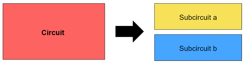
Essentially wire-cutting is exactly what the name indicates. It splits a circuit into multiple pieces by cutting one or multiple wires and moving all subsequent operations on the wire onto a new qubit [1]. Wire-cutting has a linear qubit overhead that scales with the number of cuts made. For example, a five-qubit circuit could be split into two three-qubit circuits with a single cut or two two-qubit circuits and one three-qubit circuit with two cuts. Below is a figure demonstrating how a circuit could be split using wire-cutting.

The main motivation behind wire-cutting (and other forms of circuit knitting) is increasing the number of available qubits [1] by instead of requiring larger quantum computers, introducing the concept of distributed quantum computing. In distributed quantum computing a quantum circuit too large for any single quantum computer to execute can be cut into multiple pieces. The resulting subcircuits can then be executed in parallel on multiple separate quantum computers, or, of course, sequentially on a single quantum computer.

The performance of wire-cutting is tied to the quality of the quantum hardware. Even on currently available NISQ devices, wire-cutting is showing promising results. Here, we present a simple example circuit where the result obtained on a real quantum computer using wire-cutting achieves better fidelities than the same quantum computer can achieve by just running the circuit as a whole. In addition, we use a Quantum Approximate Optimization Algorithm (QAOA) on a noisy simulator to demonstrate that even on NISQ devices, wire-cutting can improve results for real-world problems.

Theory of wire-cutting

Before advancing further into how wire-cutting works we’ll cover a few topics important for understanding it. The impatient should feel free to skip ahead to the next section to see how to use QCut with FiQCI in practice.

Quantum channel

The quantum channel technique is essentially a way to represent a transformation of a quantum state. While this may sound exactly like your normal quantum gates (and gates are also quantum channels), the difference to gates is that channels do not need to be unitary. This allows quantum channels to describe a much broader class of transformations. For example, those that require classically conditioned quantum gates such as the reset operation defined as

Even though we here perform wire-cuts without the need for reset gates and all of our operations can be implemented without classically conditioned operations, it is good to know what we mean when referring to a quantum channel below.

Quasi-probability distribution

A quasi-probability distribution is, as the name suggests, a probability distribution with some relaxed conditions. Most notably the weights of the distribution terms can be negative. They do however retain the property to yield expectation values. In circuit knitting, quasi-probability distributions are used to decompose a quantum channel into a set of quantum channels. The expectation value of the original channel can be reconstructed from the combined results of the decomposed channel. For our purposes, we will consider quasi-probability distributions as sets of quantum channels with some coefficients.

The weights for the operations are given by

\[p_1=\frac{|c_i|}{\gamma} \text{, where}\] \[\gamma = \sum_i{|c_i|},\]

where $ c_i $ are some coefficients [4].

---

With the background information covered, we move to the actual wire-cutting theory.

Quasi-Probability Distribution Simulation

Wire-cutting (and essentially all other circuit knitting) relies on quasi-probability distribution (QPD) simulation. In the context of wire-cutting this is essentially a list of quantum channels with associated coefficients of +-½ that can be used to approximate the identity channel. This means that by probabilistically applying these operations (sampling the QPD) enough times we can approximate an identity gate (an empty wire) to an arbitrary degree. The number of samples needed for an approximation of error \(\epsilon\) is given by

\[N = \gamma^{2n} \frac{1}{\epsilon^2} \text{,}\]

where n is the number of cuts made. The QPD for an identity channel is

\[Id(\bullet) = \sum_{i = 1}^{8} c_i Tr[O_i(\bullet)] \rho_i \text{,}\]

and the operations $O_i$ and $\rho_i$ can be given as [4].

$ O_i $	$ \rho_i $	$ c_i $
$ O_1 = I $	$ \rho_1 = \ket{0} \bra{0} $	$ c_1 = +1/2 $
$ O_2 = I $	$ \rho_2 = \ket 1\bra 1 $	$ c_2 = +1/2 $
$ O_3 = X $	$ \rho_3 = \ket +\bra + $	$ c_3 = +1/2 $
$ O_4 = X $	$ \rho_4 = \ket -\bra - $	$ c_4 = -1/2 $
$ O_5 = Y $	$ \rho_5 = \ket{+i}\bra{+i} $	$ c_5 = +1/2 $
$ O_6 = Y $	$ \rho_6 = \ket{-i}\bra{-i} $	$ c_6 = -1/2 $
$ O_7 = Z $	$ \rho_7 = \ket 0\bra 0 $	$ c_7 = +1/2 $
$ O_8 = Z $	$ \rho_8 = \ket 1\bra 1 $	$ c_8 = -1/2 $

An important point about notation: $ \rho_i $ are a density matrices corresponding to a state to be prepared and $ O_i $ are basis measurements, sets of operations transforming the state from one basis to another and measuring it. The identity basis here means that measurement will always yield the zero state $ \ket{0} $.

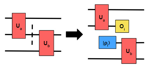
The QPD contains two types of operations. Basis measurements and state initializations. The basis measurements are inserted at the cut location and the state initializations to the beginning of the new qubit wire. For example, let’s say we have a three-qubit circuit with a Hadamard and two CNOTs that we want to cut from between the CNOTs to get two two-qubit subcircuits.

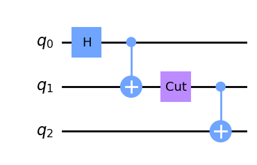
The subcircuits will then be

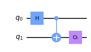
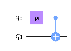
Now to be able to estimate the original circuit’s expectation values we need to insert operations from the QPD, creating a total of 8 subcircuit pairs (one for each row in the QPD ). In a more general setting, the total number of subcircuit groups of size k is given by $ 8^n $, where n is the number of cuts made and k is the number of parts the circuit is cut to. In addition to the number of circuits, also the number of samples needed scales exponentially with the number of cuts. Thus, the time complexity scales exponentially with the number of cuts. The sampling overhead can be represented in the big-O notation as O($\gamma^{2n}$) [4], where $ \gamma $ is the sum of the absolute values of the coefficients of the QPD (4 for wire-cutting). If more than one cut is made the operations for each circuit are given by the cartesian product of the QPD with itself repeated for each cut. After running all of the subcircuits on a simulator or a quantum computer we can use classical post-processing to reconstruct the expectation values.

Classical post-processing

First, it is important to notice that in our circuits we now have two kinds of measurements. The normal end-of-circuit observable measurements on the qubits we want to consider for the expectation values, and the basis measurements on the extra qubits added by wire-cuts. While the end-of-circuit measurement results are used for expectation values, the basis measurement results are used for determining coefficients for the results of each subcircuit group.

Now, once all the subcircuit groups have been run and the results collected, we can apply classical post-processing to the results. First, we choose a random circuit group result according to the QPD weights. Since for wire-cuts, the weights are all equal we just pick a random result. Then we map the measured qubit state to its eigenvalue by applying $ f:{0,1}^N \rightarrow [-1,1]^N $ [1] [4]. This means that for example, if we have 4 qubits and the states of individual qubits are [0, 1, 1, 0], we transform it to [-1, 1, 1, -1]. Next, we want to apply $ sgn(c_i)\cdot sf(\boldsymbol{y}) $ [4], where $ \boldsymbol{y} $ are the results of the end-of-circuit measurements, s the coefficient given by multiplying all the basis measurement results, and $ sgn(c_i) $ is the sign of the product of coefficients of this circuit group from the identity channel QPD. Once this has been repeated for a large enough number of times (enough samples have been collected) we can calculate the expectation value by taking the mean of the samples and multiplying it by $ (-1)^{n+1}\cdot 4^{2n} $ [4] [1], where n is the number of cuts.

Note that the above description will give the Pauli Z-observable expectation value for each qubit. If one doesn’t need the expectation value for each qubit those results can simply be ignored in the calculation. For multi-qubit expectation values after applying f the eigenvalue of a multi-qubit state is given by the product of the eigenvalues for each qubit. After which, an additional multiplication by $ (-1)^{m+1} $ where m is the number of qubits in the expectation value, is needed.

Circuit Knitting on real hardware

QCut has been designed to be compatible with the Finnish Quantum-Computing Infrastructure (FiQCI) and supports for example the 5-qubit Helmi quantum computer.

Here we demonstrate how to use QCut with FiQCI on the example circuit discussed earlier. For those interested, detailed steps can be found in a jupyter notebook at the end of this blog and more in-depth documentation is available on Github.

To use QCut (ck) we will also need some Qiskit components, such as QuantumCircuit and Estimator. We start by defining the initial and the cut circuits.

Define the initial circuit

Define the initial uncut circuit we want to execute.

circuit  =  QuantumCircuit(3)
circuit.h(0)
circuit.cx(0,1)
circuit.cx(1,2)
   
circuit.measure_all()

circuit.draw("mpl")

Insert cut operations

Add extra qubits and place cut operations to where we wish to cut the circuit.

cut_circuit = QuantumCircuit(4)
cut_circuit.h(0)
cut_circuit.cx(0,1)
cut_circuit.append(cut_wire, [1,2])
cut_circuit.cx(2,3)

cut_circuit.draw("mpl")

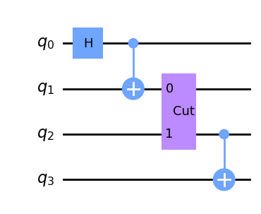
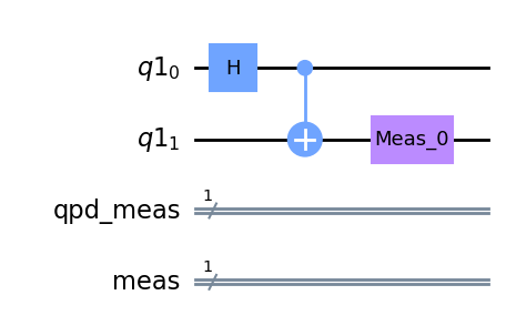
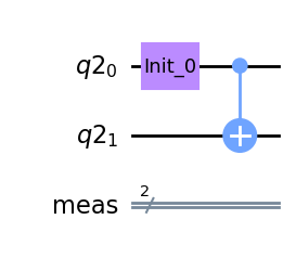
After this, we can use QCut to separate the cut_circuit from the cut location and generate all the needed experiment circuits by inserting operations from the QPD. Once we have the experiment circuits we can then execute them and estimate the expectation values of the original circuit using QCut. Here we have calculated the expectation values using the Helmi quantum computer both with and without QCut. Additionally, the expectation values have also been calculated with an ideal simulator. The separated subcircuits before inserting gates from QPD and the final results can be seen below.

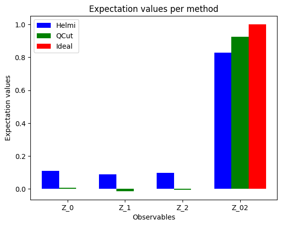
As we can see since the subcircuits use fewer qubits, have fewer gates, and are therefore less deep, they are less erroneous than the full circuit. This explains why the reconstructed expectation values are closer to the ideal ones than the ones obtained by running the full circuit.

Possible applications

Circuit knitting is a rather new tool. Potential applications for a distributed quantum computing framework utilising circuit knitting are for example VQAs, [1] [2] where one is interested in some expectation values of the system and where the circuit can be partitioned with just a few cuts. Thus, the applications depend more on the specific problem than the algorithm used, since many algorithms can have an easily cuttable form for certain problems. QAOA for the Max-Cut problem serves as a good example since for a QAOA it is easy to construct a graph that can be separated by just cutting one or two vertices [3] [5]. Here we will demonstrate solving this problem with wire-cutting on QCut and on a simulator and finally compare the results obtained to ideal ones.

QAOA max-cut with QCut

QAOA is a quantum approximation algorithm for solving combinatorial problems by optimizing some circuit parameters to obtain a minimum value for a problem-specific cost function [6]. The objective of the Max-Cut problem is to find a way to partition a graph into two separate subgraphs by cutting as many vertices as possible [7]. It has applications for example in machine learning, circuit design and statistical physics [8] [9].

Now let’s say we have a simple graph that we wish to solve the Max-Cut problem for using a QAOA.

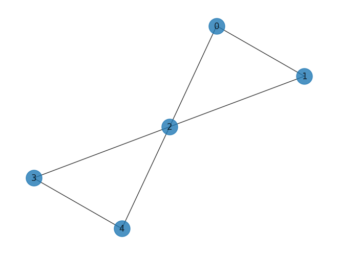
First, we need a problem Hamiltonian for this graph that describes essentially the energy of the system which we here want to minimise. For this graph the Hamiltonian is $ ZZ_{01} + ZZ_{02} + ZZ_{12} + ZZ_{23} + ZZ_{24} + ZZ_{34} $ Here $ ZZ_{ij} $ are RZZ-rotation gates and i, and j are some qubit indices. You can see that each RZZ-gate here corresponds to a vertex in the graph. Now this Hamiltonian can be converted to a circuit by taking the terms as gates. This gives us the circuit below. Now this Hamiltonian is our cost function and its expectation value is what we want to minimise by finding appropriate parameters for the RZZ-gates. In addition to the cost Hamiltonian, we also need a mixer Hamiltonian that stops us from getting stuck in a suboptimal state. Here the mizer consists of applying RX-gates on each qubit. We will choose initial parameters of $ [-\pi, -\pi] $. Here we will use the scipy.minimize() function using the COBYLA method to minimize the cost function.

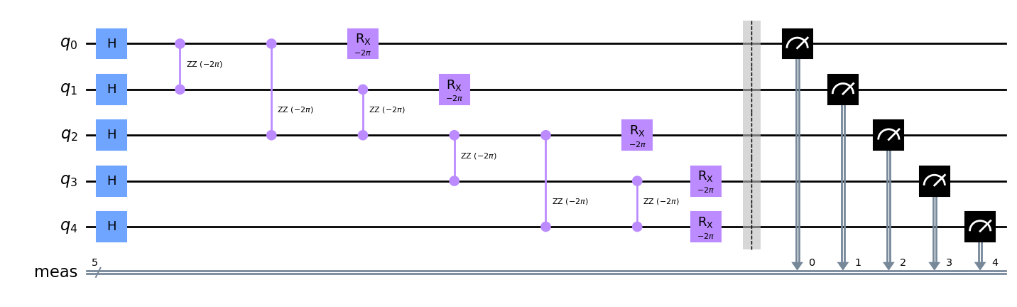
We can see that the circuit is structured in a way where we can easily cut a wire on the second qubit to split it in two. This is shown in the circuit below. After this, the QCut wire-cutting procedure can be executed just like we did above.

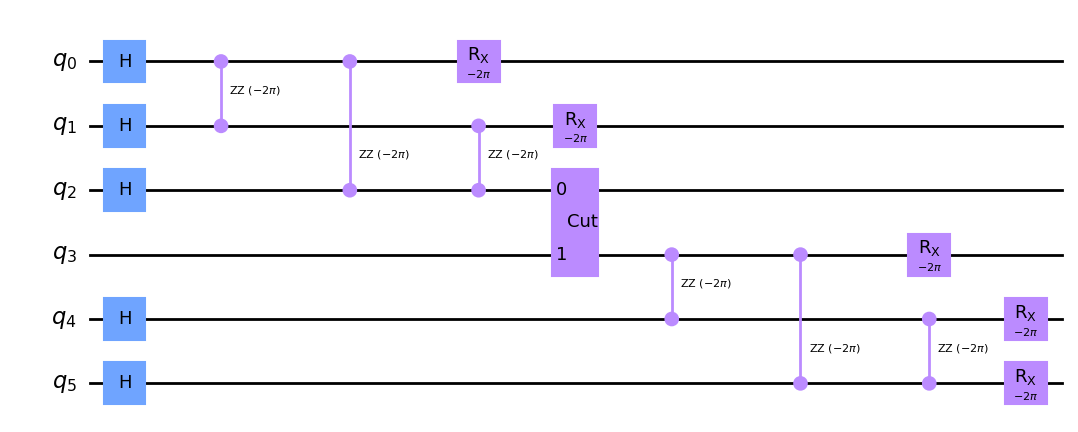
In the circuit, you can notice that the parameters are $ -2\pi $ instead of $ -\pi $ This is just because when constructing the circuit we multiply the parameters by 2. This is just a convention and does not affect our results.

Now that we have our cost function and circuit we can solve the problem. A notebook with more details is provided at the end of the blog.

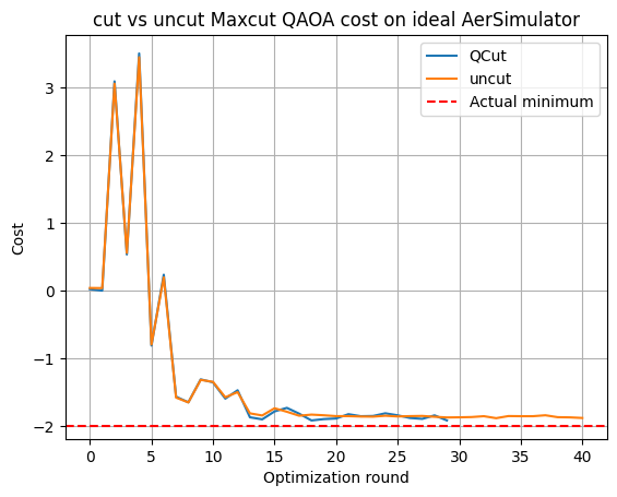
Results

Solving the QAOA with Qiskits AerSimulator as our backend we can see that the results obtained are very close to the true minimum of -2 and that QCut can accurately estimate the cost function.

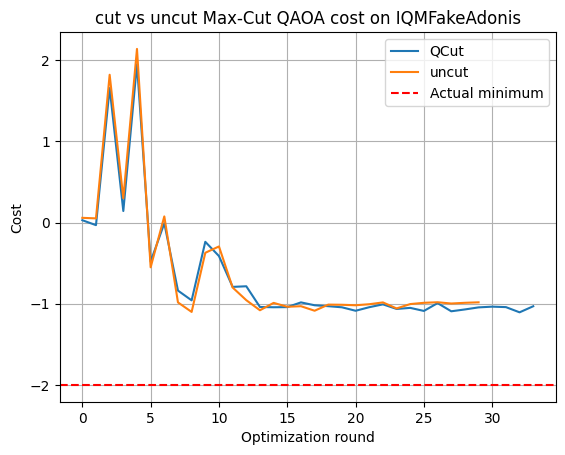
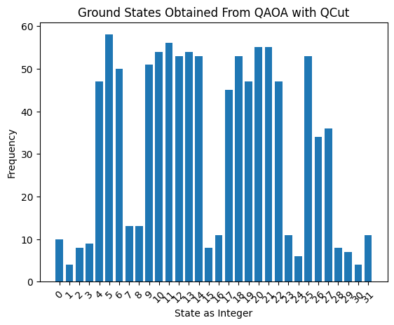
When running with the IQMFakeAdonis backend that models the noise of the Helmi quantum computer we see that neither the uncut QAOA nor the one cut with QCut reach the true minimum. The results from QCut again closely match the results obtained with the noisy simulator. Even though the accurate minimum cost is not reached, the optimal parameters reached with QCut are good enough to accurately obtain all of the solution states to the Max-Cut problem. Thus QCut could be used to accurately solve similar optimization problems requiring more qubits than available on the physical hardware.

One can see that the ideal solution states [4, 5, 6, 9, 10, 11, 12, 13, 14, 17, 18, 19, 20, 21, 22, 25, 26, 27] have the highest probabilities to be measured. The ideal solution states were calculated with the openQAOA python package.

So even though the results are erroneous, with QCut they are of sufficient quality to accurately solve the problem.

Results and Outlook

Results for wire-cutting, and circuit knitting in general, are very encouraging and show the potential utility of distributed quantum computing. Such a framework would allow solving huge problems, by splitting the task across multiple quantum computers, increasing the number of available qubits past the number of qubits on the largest individual quantum computer. This, of course, is only possible given advanced enough hardware. However, as we have demonstrated here, wire-cutting could prove useful even on noisy hardware. By splitting the circuit of interest into smaller chunks, the accumulated error can be significantly reduced.

However, it is good to note that circuit knitting has an exponential overhead in the number of circuits needed, which scales with the number of cuts made. How useful circuit knitting will be, and for which types of problems it is suitable, time will tell. Currently, the runtime overhead that comes from the additional circuits needed for circuit knitting is amplified by the limited availability of quantum computers, which prevents full parallelization of the problem over several QPUs. With the possibility to send each, or a few, subcircuits to separate QPUs would significantly reduce the overall wall-time for solving a given problem, even if the total QPU time would remain the same.

Notebooks

The notebooks used can be accessed here.

For more examples on wire-cutting with QCut check it out on Github.

References

1. T. Peng, A. W. Harrow, M. Ozols, and X. Wu, “Simulating Large Quantum Circuits on a Small Quantum Computer,” Phys. Rev. Lett., vol. 125, no. 15, p. 150504, Oct. 2020, doi: 10.1103/PhysRevLett.125.150504. Available: https://link.aps.org/doi/10.1103/PhysRevLett.125.150504. [Accessed: Aug. 14, 2024]

2. G. Gentinetta, F. Metz, and G. Carleo, “Overhead-constrained circuit knitting for variational quantum dynamics,” Quantum, vol. 8, p. 1296, Mar. 2024, doi: 10.22331/q-2024-03-21-1296. Available: https://quantum-journal.org/papers/q-2024-03-21-1296. [Accessed: Aug. 14, 2024]

3. M. Bechtold et al., “Investigating the effect of circuit cutting in QAOA for the MaxCut problem on NISQ devices,” Quantum Sci. Technol., vol. 8, no. 4, p. 045022, Oct. 2023, doi: 10.1088/2058-9565/acf59c. Available: https://iopscience.iop.org/article/10.1088/2058-9565/acf59c. [Accessed: Aug. 14, 2024]

4. H. Harada, K. Wada, and N. Yamamoto, “Doubly optimal parallel wire cutting without ancilla qubits.” arXiv, Nov. 07, 2023. doi: 10.48550/arXiv.2303.07340. Available: http://arxiv.org/abs/2303.07340. [Accessed: Aug. 14, 2024]

5. G. Uchehara, M. Medvidovic, and A. Apte, “Quantum Circuit Cutting,” PennyLane Demos, Sep. 2022, Available: https://pennylane.ai/qml/demos/tutorial_quantum_circuit_cutting/#lowe2022. [Accessed: Aug. 14, 2024]

6. L. Zhou, S.-T. Wang, S. Choi, H. Pichler, and M. D. Lukin, “Quantum Approximate Optimization Algorithm: Performance, Mechanism, and Implementation on Near-Term Devices,” Phys. Rev. X, vol. 10, no. 2, p. 021067, Jun. 2020, doi: 10.1103/PhysRevX.10.021067. Available: https://link.aps.org/doi/10.1103/PhysRevX.10.021067. [Accessed: Aug. 14, 2024]¨

7. M. X. Goemans and D. P. Williamson, “Improved approximation algorithms for maximum cut and satisfiability problems using semidefinite programming,” J. ACM, vol. 42, no. 6, pp. 1115–1145, Nov. 1995, doi: 10.1145/227683.227684. Available: https://dl.acm.org/doi/10.1145/227683.227684. [Accessed: Aug. 14, 2024]

8. Y. Y. Boykov and M.-P. Jolly, “Interactive graph cuts for optimal boundary \& region segmentation of objects in N-D images,” in Proceedings Eighth IEEE International Conference on Computer Vision. ICCV 2001, Vancouver, BC, Canada: IEEE Comput. Soc, 2001, pp. 105–112. doi: 10.1109/ICCV.2001.937505. Available: http://ieeexplore.ieee.org/document/937505. [Accessed: Aug. 14, 2024]

9. F. Barahona, M. Grötschel, M. Jünger, and G. Reinelt, “An Application of Combinatorial Optimization to Statistical Physics and Circuit Layout Design,” Operations Research, vol. 36, no. 3, pp. 493–513, Jun. 1988, doi: 10.1287/opre.36.3.493. Available: https://pubsonline.informs.org/doi/10.1287/opre.36.3.493. [Accessed: Aug. 14, 2024]

Give feedback!

Feedback is greatly appreciated! You can send feedback directly to fiqci-feedback@postit.csc.fi.