Quantum k-means for clustering and segmenting satellite images

2024-08-22 14 minute read

Machine learning is used to process and analyze different types of datasets for example to extract information and make predictions about the data. Machine learning algorithms can be used in image processing, filtering, image segmentation, clustering, or signal processing. These algorithms become heavy to run as they consume plenty of computational resources when the complexity and amount of data increases [1,2]. Working with large amounts of data has become more and more important for multiple industries [3]. One example is the field of Earth observation, where for example satellite image data needs to be analyzed [2,4]. The images can contain high amounts of information depending on what is being researched and how.

The use of quantum computers and quantum algorithms have been proposed for decreasing the processing requirements of machine learning algorithms and to make them more efficient when processing complex data sets [2,4,5]. Combining quantum algorithms with classical machine learning algorithms could provide speed-ups or other enhancements to the machine learning workflows. The power of quantum algorithms comes from the possibility of processing multiple inputs in parallel, capturing complex dependencies in the data, speeding up linear algebra, and operating with high-dimensional data. These properties stem from concepts of quantum mechanics like superposition and entanglement. Thus, quantum computers could make working with complex and large data sets significantly more efficient.

In this blog post, the main focus is to investigate the k-means algorithm which can be used to cluster and segment images. The k-means was chosen because of the conceptual simplicity of the algorithm and the versatile use cases of clustering algorithms. Here, a quantum k-means algorithm, which is a quantum-enhanced version of the classical k-means algorithm, is created and its performance is tested. The testing is done by clustering a dataset of satellite images and segmenting satellite images. This practical example was chosen because the data sets used for Earth observation can be very large. It is also a field that already uses machine learning and could thus directly benefit from advancements in machine learning provided by quantum enhancements.

Here, we use the EuroSAT dataset [1], a dataset of 27 000 labeled images from the Sentinel-2 satellite. The dataset is used for classifying land use and land coverage. It is available in RGB and multi-spectral versions. In this example, we use the RGB version, as it is a bit easier to work with. Figure 1 shows an example of two types of images in the dataset.

Previously, the EuroSAT data set has been classified with a quantum convolutional neural network (QCNN) [2] and parameterized quantum circuits (PQC) [3]. These approaches usually lead to more complicated circuits and require more qubits compared to the quantum k-means method. QCNN and PQC also need to be trained, while the k-means does not.

Example of an image that is labeled as Residential

Example of an image that is labeled as Forest

Figure 1: Two examples of the satellite images that are in the EuroSAT dataset. The complete dataset contains ten different categories of images and some of the other labels are for example AnnualCrop, Highway, River, and Industrial.

In what follows, we first go through the basics of the classical k-means algorithm, and then present a version of a quantum k-means algorithm. We then describe the clustering and segmentation tests and analyze the results. The code used for the quantum k-means can be found in the Jupyter notebooks linked at the end of this blog post. The notebooks provide more information about the construction of the algorithm and some mathematical explanations of the steps.

Basics of the Classical K-means Algorithm

Firstly, what is k-means? K-means is an unsupervised machine learning algorithm [4,5]. It takes $n$ vectors and divides them into $k$ groups. The clustering is done by calculating the distance between a vector and each of the cluster centroids and assigning the vector to the nearest cluster. This is repeated for every vector. After each vector has been assigned to a cluster, new centroids are determined based on the mean of the vectors in a cluster. Now, the distances between the vectors and the new centroids are calculated and a vector is possibly moved to a new closer cluster. This is repeated until the centroids of the clusters do not change after computing the mean of the cluster.

The algorithm becomes computationally heavy as the number and the dimension of the vectors grow. According to [5], the heaviest part of the k-means is calculating the distance between each vector and each cluster centroid. In [4] the time complexity of this algorithm is given as $O(Nnk)$, where $N$ is the number of features in the vector, $n$ is the number of vectors, and $k$ is the number of clusters. The time complexity describes the computing time required to run a certain algorithm, and ideally this should be minimized.

The Quantum K-means Algorithm

How can a quantum computer be used in this? Well, for example, a quantum computer could be used to perform some of the steps in the k-means algorithm. In the algorithm that is described in this blog, the distance calculation is done with a quantum circuit that is then run on Helmi, a 5-qubit quantum computer connected to the LUMI-supercomputer, a part of the Finnish Quantum Computing Infrastructure (FiQCI)

Thus, the k-means algorithm will be similar to the classical algorithm regarding the initialization of the centroids, cluster assignment, and updating of the clusters, but the distance to determine in which cluster a vector belongs is computed with a quantum circuit. The steps in building this circuit include encoding the vectors into the qubits and then building a circuit to compute the distance. Both of these can be done in several different ways. Here, amplitude encoding was chosen to store the information from the vectors into the qubits, and the swap test was chosen for the distance calculation, as presented by Dawid Kopczyk in [5].

To classify the vectors with a quantum circuit we need to embed their information into the qubits. One way to do so is with amplitude encoding. This means that the vector is normalized and the points from it are used as amplitudes of the initial states of the qubits. Amplitude encoding has previously been presented for example in [4,6,7]. In this example, a function to do this is created and the state vectors $\phi$ and $\psi$ that it gives are done as described in [5]. The state $\ket{\phi}$ has one qubit allocated to it and $\ket{\psi}$ has $\log_2{l}$ number of qubits, where $l$ is the length of the state vector $\psi$. The length of the state vector $\psi$ depends on the number of dimensions of the data.

Kopczyk also presents one of the most common ways of finding the similarity between two quantum states, the swap test. The swap test is a simple quantum circuit where the ancilla qubit is put into superposition with a Hadamard gate, then the controlled swap gate is used with the ancilla qubit as the control qubit, and before measuring the ancilla a Hadamard gate is reapplied. Thus, the number of qubits that are needed to perform this algorithm is one for the ancilla, one for the state $\ket{\phi}$ and the amount of qubits in the state $\ket{\psi}$ . Figure 2 shows the circuit diagram.

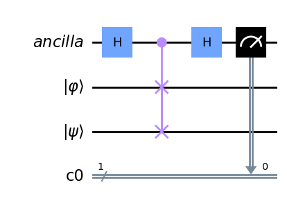
Figure 2: The circuit diagram of the swap test used to compute the similarity between two quantum states.

After applying the swap test to the quantum circuit, the similarity of the states can be derived from the probability of the ancilla qubit being $0$. The probability is of the form $P(\ket{0})= \frac{1}{2} + \frac{1}{2}\vert \braket{\phi \vert \psi} \vert^2$ , where the last inner product is the fidelity of the states [8]. The fidelity represents the probability that one quantum state is identified as the other. More detailed descriptions of how this leads to the Euclidean distance of two vectors can be found with the code in the Jupyter Notebook. After the distance between a vector and a cluster centroid is calculated the rest of the algorithm is computed classically.

This way of implementing the quantum k-means algorithm gives the time complexity of $O(log(N)nk)$ [4]. Thus, compared to the classical algorithm the distance calculation part of the k-means is sped-up exponentially with the quantum implementation.

Testing the Quantum K-means for Clustering

To test the quantum k-means algorithm for clustering, ten different data sets with ten images in each are clustered. Each data set has images only from the categories Forest and Residential and the clustering is done into two clusters. With smaller data sets the computing time can be used more efficiently and more examples can be compared to each other.

To prepare the images for the clustering, they are passed through a pretrained feature extraction model, the VGG16, and the features are reduced with principal component analysis (PCA). The VGG16 is a convolutional neural network developed by the Visual Geometry Group at the University of Oxford. PCA is a commonly used unsupervised machine learning algorithm for feature reduction. PCA and VGG16 have been shown to enhance the performance of a clustering algorithm and they have previously been used in quantum implementations [3,9,10].

To run the quantum algorithm on the Helmi quantum computer with just five qubits, small and simple data is preferred. Thus, all of the data sets used were reduced to have only one dimension, that is, one feature. Then each data set was clustered with Helmi. Even if the data structure in this example is simple, the algorithm is scalable and can be used for larger data sets with a greater number of features and the clustering can be done to more than two clusters.

In the end, the correctness of the clustering is evaluated with the adjusted rand index (ARI). It is a function from Scikit-learn that computes the similarity between the true and predicted labels of the clusters [11]. The ARI score can be defined as:

\[ARI = \frac{RI - ExpectedRI}{maximum(RI) - ExpectedRI}\]

where $RI = \frac{TP + TN}{TP + FP + FN + TN}$

The $RI$ is the rand index that is defined with true positives $(TP)$, true negatives $(TN)$, false positives $(FP)$, and false negatives $(FN)$.

The score ranges from $-0.5$ to $1$, where $1$ stands for perfect clustering, $0$ is random clustering, and $-0.5$ is worse than random clustering. The ARI score from the quantum k-means is compared to the ARI score of the classical k-means for each data set.

Results of the Quantum K-means Clustering

After the clustering algorithm has been run for each data set, the ARI scores for the quantum and the classical k-means can be compared. All of the ARI scores can be seen in Table 1 and the average ARI scores for both algorithms are in Table 2. The most common result was both algorithms getting an ARI score of $1$. The quantum algorithm outperformed the classical one by getting a higher ARI score for three data sets. The quantum k-means was also run on some bigger data sets, with more data points and more features, and the results were coherent with this. The quantum algorithm usually performed as well as the classical one.

Table 1: The quantum and classical ARI scores from clustering all ten data sets. The ARI scores were obtained after running the quantum k-means algorithm on the Helmi quantum computer.
Data set	Quantum ARI score	Classical ARI score
Data set 1	1.0	1.0
Data set 2	1.0	1.0
Data set 3	1.0	1.0
Data set 4	1.0	0.597
Data set 5	1.0	1.0
Data set 6	0.597	0.294
Data set 7	1.0	1.0
Data set 8	1.0	0.597
Data set 9	1.0	1.0
Data set 10	1.0	1.0

Table 2: Comparison of the ARI scores from Table 1.
	Average
Classical ARI score	0.8488
Quantum ARI score	0.9597

The clusters can also be visualized by plotting. Figure 3 shows the results from the quantum and classical algorithms for three different data sets. The plots show each point in the cluster it has been assigned to and the two clusters can be differentiated by the color of the points and by the label value on the y-axis.

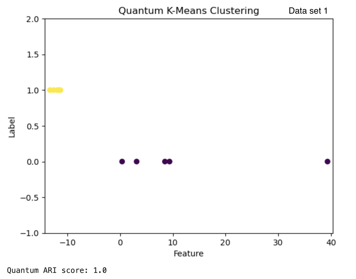
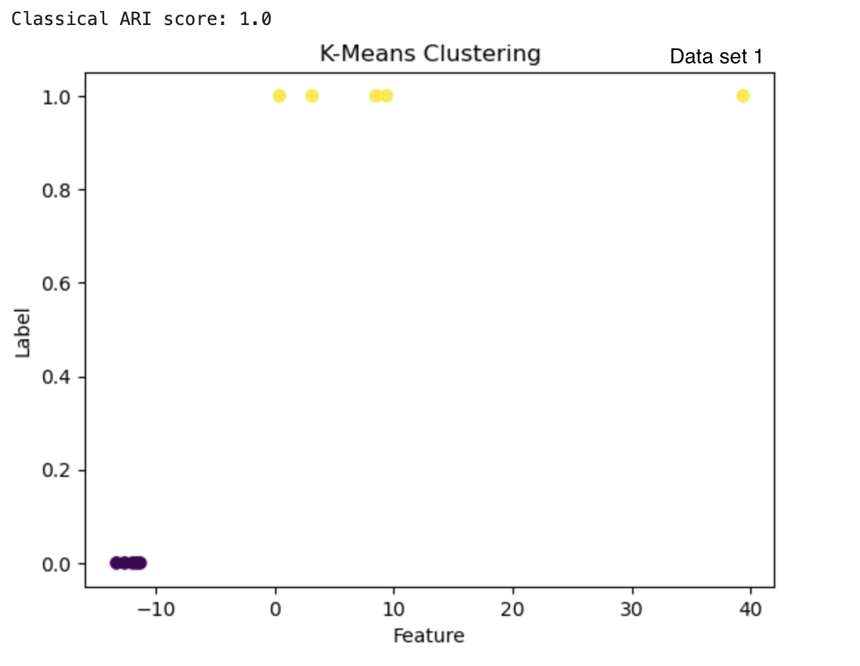
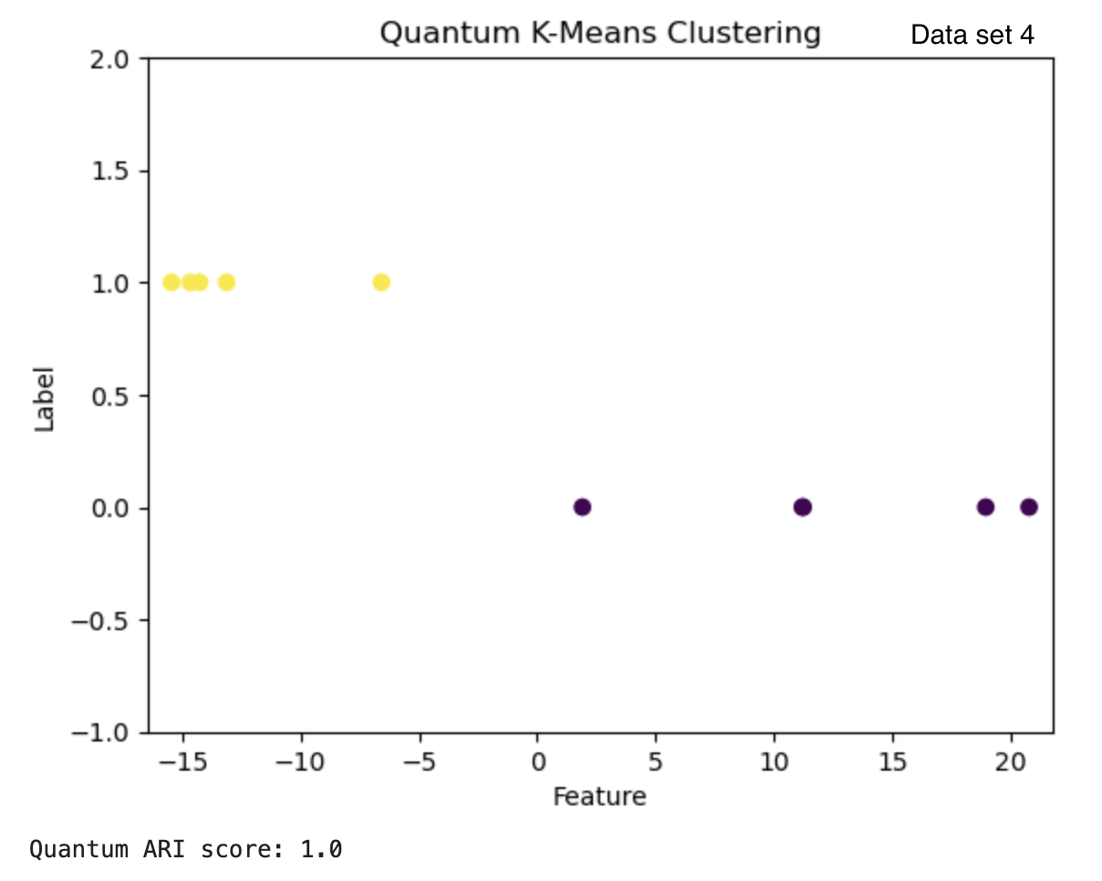
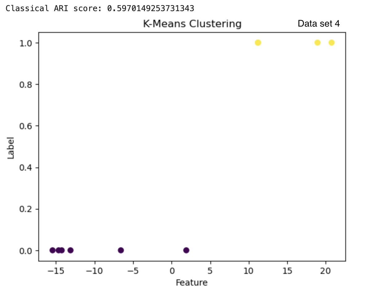
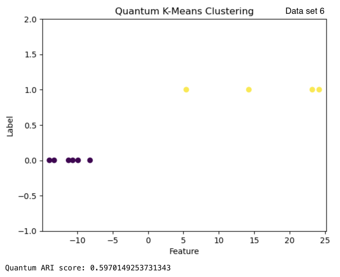
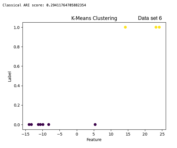
Figure 3: The results from the quantum k-means are on the left with the ARI score below each clustering result. The results from the classical algorithm are on the right with the ARI score above each clustering result. The graphs have the feature of the vectors on the x-axis and the cluster label on the y-axis.

Each point in the cluster can be traced back to the image that it represents. The images can be plotted based on the predicted labels they have. Figure 4 shows the images of one data set clustered into two groups. The true and predicted labels for each image are also visible.

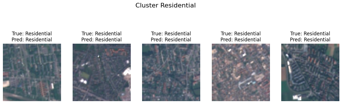
(a) The images of residential areas with their true and predicted labels.

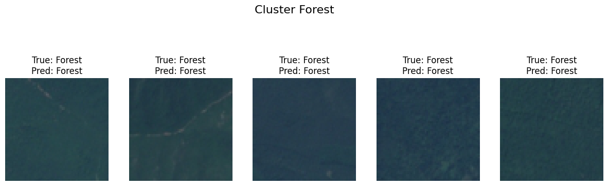
(b) The images of forest with their true and predicted labels.

Figure 4: After clustering the vectors, the images from each cluster can be plotted and the true and predicted labels can be compared. In (a) and (b) you can see images clustered into the Residential and Forest clusters.

Testing the Quantum K-means for Image Segmentation

Besides the clustering, the quantum k-means algorithm can be used for image segmentation. To segment an image from the EuroSAT data set it was transformed into a two-dimensional array that contains each pixel and the array of the RGB values in that pixel. Then, the images were changed to gray-scale and flattened into a one-dimensional array of the pixel values. Thus, the distance between the pixels will be the difference in their intensity. The distance of the points was then determined with the same quantum circuit that uses the swap test. Using a swap test in image segmentation has been previously done in [10].

Compared to the clustering of the images, in this version of the quantum k-means the distance of the points from each other was only determined by the similarity of the states provided by the probability of the ancilla being in state $0$ and not the Euclidean distance between the pixels. Otherwise, the algorithm is the same as for the clustering task. The algorithm was tested on some images from different categories of the EuroSAT data set. The code for this algorithm is also available.

For demonstration purposes, the quantum k-means for the image segmentation was run on a simulator. Nevertheless, the code is the same as for the clustering tests run on a real quantum computer.

Results of the Quantum K-means Image Segmentation

The results of the image segmentation done with the quantum k-means algorithm can be seen in Figure 5. The segmented images represent the original images quite closely and they can be used for different purposes. For example, different areas of land usage are well visible, height differences of the land can be visualized, and roads, buildings, and rivers can be recognized from the surrounding environment.

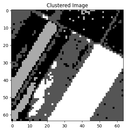
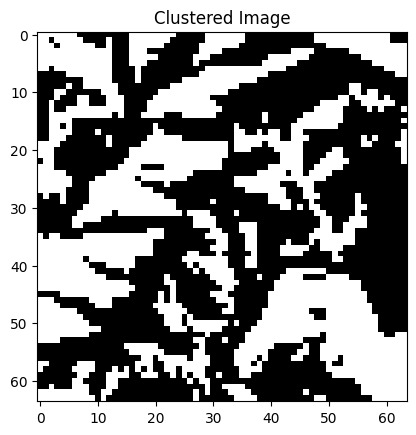
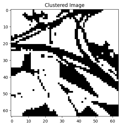
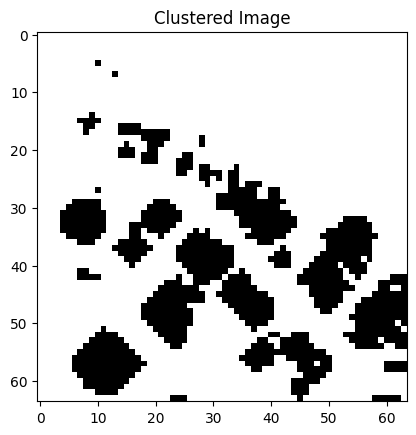
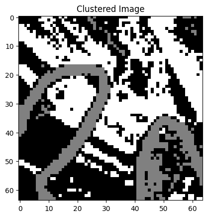
Figure 5: Some satellite images from the EuroSAT data set and their segmented versions. The segmentation has been done with the quantum k-means algorithm. The left most image has been segmented into four clusters, the right most images into three clusters and the rest have two clusters.

Conclusion and Outlook

Machine learning algorithms can indeed benefit from quantum computing. Even on the current noisy quantum computers, the quantum k-means algorithm can attain as accurate or more accurate results than the fully classical k-means when they are used for clustering satellite images from the EuroSAT data set. The use of quantum k-means is also versatile as it can be applied to image segmentation in addition to clustering.

Future steps in combining machine learning algorithms with quantum computing could include implementing more of the parts of the algorithm with quantum circuits, like searching for the closest cluster could be done with a quantum algorithm like Grover’s algorithm [12]. Implementing machine learning algorithms with QCNNs could also be beneficial once more qubits are available. With the continuously increasing capacity of quantum computers, the quantum k-means can be used for bigger data sets. At some point, it is expected that a quantum-enhanced solution is faster and/or more accurate compared to a purely classical algorithm.

Notebooks

The Jupyter Notebooks with more information about the algorithm and the codes to run the quantum k-means algorithm for clustering and image segmentation can be found here.

They can be executed directly on the FiQCI infrastructure.