Cutting circuits#

Import needed packages#

import numpy as np
import QCut as ck
from QCut import cut, cutGate, CutOptions, find_cuts
from qiskit import QuantumCircuit, transpile
from qiskit.circuit.library import CXGate
from qiskit.quantum_info import SparsePauliOp
from qiskit_aer import AerSimulator
from qiskit.primitives import StatevectorEstimator as Estimator, BackendEstimatorV2 as BackendEstimator
from iqm.qiskit_iqm import IQMFakeAdonis

Define a QuantumCircuit just like in Qiskit#

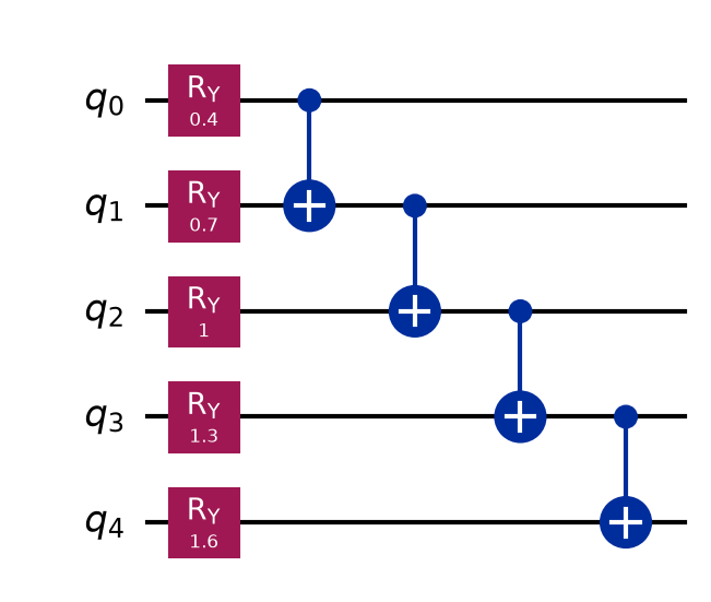
circuit = QuantumCircuit(5)

for qubit in range(5):
    circuit.ry(0.4 + 0.3*qubit, qubit)
circuit.cx(0,1)
circuit.cx(1,2)
circuit.cx(2,3)
circuit.cx(3,4)

circuit.draw("mpl")

Insert cuts to denote where to cut the circuit#

Note that here we don’t insert any measurements. Measurements will be automatically handled by QCut.

marked_circuit = QuantumCircuit(5)

for qubit in range(5):
    marked_circuit.ry(0.4 + 0.3*qubit, qubit)
marked_circuit.cx(0,1)
marked_circuit.append(**cutGate(CXGate(), 1, 2))
marked_circuit.cx(2,3)
marked_circuit.append(cut(), [3])
marked_circuit.cx(3,4)

marked_circuit.decompose(gates_to_decompose=["CutGate"]).draw("mpl")

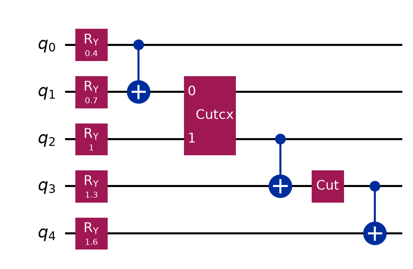
cutGate() marks a gate cut and cut() a wire cut. Any two-qubit gate can be cut, with the decomposition derived from the gate’s KAK coordinates, so the CX above is a single cut rather than a CZ with fix-up gates around it. See gate cuts and wire cuts for more on placing them, and Theory for where the decompositions come from.

Extract cut locations and split into independent subcircuits#

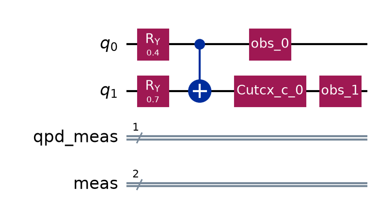
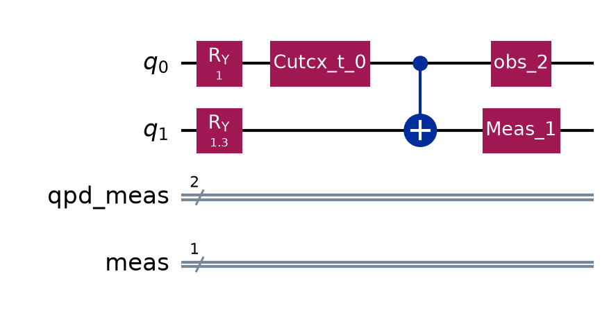
cut_circuit = ck.get_locations_and_subcircuits(marked_circuit)

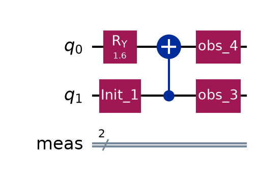
Now we can draw our subcircuits.

cut_circuit.subcircuits[0].draw("mpl")

cut_circuit.subcircuits[1].draw("mpl")

cut_circuit.subcircuits[2].draw("mpl")

Define observables and generate experiment circuits#

Observables are given the way Qiskit’s estimator takes them: a Pauli label, a Pauli, a SparsePauliOp, a SparseObservable (qiskit 2.1+), a {label: coefficient} mapping, or any nested sequence of those. The expectation values come back shaped like what you pass, so a list of four observables gives four values, in order. See Defining observables for more.

observables = ["IIIIZ", "IIIZI", "IIZII", "IIIZZ"]

cut_experiment = ck.get_experiment_circuits(cut_circuit, observables)

print(cut_experiment.num_groups)

48

get_experiment_circuits() does not modify the CutCircuit it is given, so the same split can be reused for several observable sets. Both CutCircuit and CutExperiment implement the assign_parameters() function of Qiskit.QuantumCircuit.

What a cut costs#

print(cut_circuit.gamma, cut_circuit.optimal_gamma)

12.0 9.0

gamma is the sampling overhead of this split and optimal_gamma the least those same cuts could cost with every decomposition available. Shot cost goes as gamma squared. Both are closed form, so a plan can be costed before any experiment circuits are built, and CutExperiment carries both forward.

The gap here is the lone wire cut: on its own it does not communicate under the default wire_cut_communication="auto", so it costs 4 rather than 3. Passing "always" closes it and this split reaches 9.

Cheaper decompositions#

Cuts are not decomposed one at a time where a cheaper joint decomposition exists. All three of the below are on by default and can be turned off through Options.

	default	turned off
A run of gates on one qubit pair costs a single cut	1 cut, gamma 1.59, 6 subexperiments	2 cuts, gamma 9, 36
Parallel single-axis rotations share one decomposition (derivation)	gamma 5.50, 30 subexperiments	gamma 6.77, 36
A block of parallel wire cuts exchanges its measured outcome (derivation)	gamma 7, 28 subexperiments	gamma 16, 64

A separate circuit, to show the last of those on its own. Two parallel wire cuts cost 2**(n+1) - 1 rather than 4**n:

pair = QuantumCircuit(4)
for qubit in range(4):
    pair.ry(0.4 + 0.2 * qubit, qubit)
pair.cx(0, 1)
pair.cx(0, 2)
pair.append(cut(), [1])
pair.append(cut(), [2])
pair.cx(1, 2)
pair.cx(2, 3)

block = ck.get_locations_and_subcircuits(pair)
local = ck.get_locations_and_subcircuits(
    pair, options=CutOptions(wire_cut_communication="never")
)

print(block.gamma, local.gamma, local.optimal_gamma)

7.0 16.0 7.0

Those cuts run in waves, since one side has to be measured before the other can prepare what it measured. submit_experiments() handles that itself.

Options#

CutOptions is collected once and carried through the run. It covers the three decompositions above, the expansion strategy, sampling and the cut finder. Above 1000 groups the experiment is sampled from the quasiprobability distribution rather than enumerated. Every option and its default is listed under Options.

Automatic cuts#

QCut comes with functionality for automatically finding good cut locations that can place both wire and gate cuts.

options = CutOptions(
   finder_num_partitions=3,
   finder_cut_mode="both",
)

found = find_cuts(circuit, options=options)

print(len(found.cut_locations), found.gamma)

2 9.0

Here the finder reaches the optimal_gamma the hand-placed cuts above did not. See automatic cuts for the finder’s own options and how it chooses.

In depth#

Each kind of cut has a page of its own, with its own setup.

Cutting circuits

Contents