
The FiQCI software stack has been extended with a simple-to-use quantum error mitigation service (EMS). The EMS offers users the ability to easily add error mitigation methods to quantum jobs submitted through LUMI and executed on VTT Q50. Currently, the service supports, for example, readout error mitigation (REM) as an error mitigation method in post-processing. This can be applied either automatically or manually. The automatic mode aims for ease of use and minimal effort from the user, while the manual method offers more control. This notebook focuses on REM but EMS also provides utilities similar to the qiskit primitives (Sampler and Estimator) for sampling and expectation value calculation. In addition to REM these utilities support dynamical decoupling, Pauli twirling, and zero-noise extrapolation. For more info on EMS see FiQCI EMS Documentation.

What Is Error Mitigation and Why Is It Needed?
Current quantum computers are in the noisy intermediate-scale quantum (NISQ) era. They have a qubit count ranging from tens to hundreds of qubits, noise affects performance, and they do not yet support full quantum error correction (QEC). Various methods for dealing with noise and errors on quantum computers are under active development, many of which are usable on NISQ devices.
These methods can be divided into three different categories: error suppression, error mitigation, and error correction. Error suppression refers to techniques used actively during the execution of the quantum circuit to lower the probability of an error occurring. For example, so-called dynamic decoupling is an error suppression method. Error mitigation refers to techniques used to mitigate or lessen the effects of the errors after the circuit has been executed in the post-processing step. Methods include readout error mitigation and zero-noise extrapolation. Error correction in turn refers to methods used to identify and correct errors during the execution of a quantum circuit. 1
Here, we first go through what readout error mitigation is and then give a usage example of applying readout error mitigation on the FiQCI infrastructure. At the end of the blog post references and additional resources are given.
Readout Error Mitigation
Imagine a faulty scale that consistently reads 1 kg too heavy. You do not necessarily need a better scale, you just need to know about the bias so you can subtract it from every reading. Readout error mitigation works similarly: instead of fixing the noisy measurement hardware, we first characterize how it tends to misbehave, and then correct for that bias in software after the fact.
Readout error mitigation is thus a technique used to mitigate errors caused by imperfect measurements, which are one of the major sources of errors in current quantum computers. Specifically, readout error mitigation aims to correct measurement errors in which a qubit is reported as being in state $\ket{1}$ when its true state is $\ket{0}$, and vice versa. The basic idea behind this technique is to characterize the probabilities of observing each qubit in the correct and incorrect states. 2 These probabilities can be obtained in several ways, for example, by running two quantum circuits to characterize the measurement errors. One circuit measures the qubits after each has been initialized to state $\ket{0}$ but before any quantum gates are applied to them, and the other circuit also initializes the qubit to state $\ket{0}$ and then applies an X gate to each qubit after which the qubits are measured. Hence, for the case of the first circuit, all qubits should be measured in the state $\ket{0}$ and, for the case of the second circuit, all qubits should be measured in the state $\ket{1}$. This way the probabilities $P(0\mid 0)$, $P(0\mid 1)$, $P(1\mid 0)$, and $P(1\mid 1)$ are determined for each qubit, where, for example, $P(1\mid 0)$ denotes the probability of observing $\ket{1}$ when the qubit’s true state was $\ket{0}$. This method assumes that the measurement errors are uncorrelated and that the X gate itself is error-free; a reasonable but imperfect approximation. 3
The most straightforward way to apply readout error mitigation is to build a so-called confusion matrix from these probabilities and use it to correct the raw counts in post-processing. A one-qubit confusion matrix, $A_k$, has the general form
\[A_k = \begin{bmatrix} P_k(0\mid 0) & P_k(0\mid 1) \\ P_k(1\mid 0) & P_k(1\mid 1) \end{bmatrix},\]where the notation $P_k(i\mid j)$ denotes the probability of observing qubit $k$ in the state $\ket{i}$ when the true state is $\ket{j}$. Assuming that the readout errors of each qubit are independent, a $2^n\times 2^n$ confusion matrix $A$ for an n-qubit system can be constructed from $n$ independent $2\times 2$ confusion matrices $A_k$ as \(A = A_1 \otimes A_2 \otimes \ldots \otimes A_n.\) This confusion matrix $A$ can be used to describe a relation between the ideal and noisy measurement results \(p_{\mathrm{noisy}} = Ap_{\mathrm{ideal}},\) where $p_{\mathrm{noisy}}$ and $p_{\mathrm{ideal}}$ are output probability vectors. 4
Similarly to how the confusion matrix can be used to obtain the noisy probability vector from the ideal one, the Moore-Penrose pseudoinverse $A^+$ of the confusion matrix $A$ can be used to obtain the mitigated probability vector \(p_{\mathrm{mitigated}} = A^+p_{\mathrm{noisy}}.\) It is sufficient to construct the confusion matrix and its pseudoinverse once per calibration cycle as the readout error rates are relatively stable. 4
Even though this is the most straightforward way to apply readout error mitigation, it is not how EMS applies readout error mitigation as the REM method in FiQCI EMS is based on Matrix-free measurement mitigation 5.
As the confusion matrix scales as $2^n \times 2^n$, performing readout error mitigation by building the full confusion matrix is feasible only for small QPUs or when readout error mitigation is applied to a small set of qubits. However, there are methods to overcome this scaling issue. For example, one option is to use a reduced confusion matrix $\tilde{A}$, which is the approach used by IBM’s Mthree (matrix-free measurement mitigation). We follow this approach through IQM’s Mthree adapter.
This reduced confusion matrix is a $k \times k$ matrix, where $k$ is the number of unique bit-strings obtained from the noisy measurements. This value $k$ is typically much smaller than $2^n$, especially when $n$ is large (i.e., for high-qubit-count QPUs). The key idea behind the reduced confusion matrix is that any bit-string which never appeared in the noisy measurements is also assumed to never appear in the ideal (noise-free) distribution. In other words, the set of bit-strings in $p_{\mathrm{ideal}}$ is treated as a subset of those observed in $p_{\mathrm{noisy}}$. 2, 4
To make this concrete: suppose the noisy measurements produced only the bit-strings $000, 010, 011,$ and $111$. Since $001, 100, 101,$ and $110$ were never observed, they are assumed not to be plausible ideal outcomes either. The reduced confusion matrix is therefore built to only describe transitions between the observed bit-strings, and any correction terms that would map a noisy outcome to one of the unobserved strings are dropped entirely. This is what keeps the matrix at size $k \times k$ rather than $2^n \times 2^n$.
However, sometimes even the reduced confusion matrix $\tilde{A}$ is still too large or too expensive to construct. 2 For these cases, Mthree uses iterative methods (GMRES with Jacobi preconditioning) to solve systems of linear equations to correct the noisy outcomes to the ideal outcomes. The usage of these iterative methods is possible because the elements of the single-qubit confusion matrices $A_k$ are stored individually and hence can be accessed. 6
Usage Example
When readout error mitigation is applied using the FiQCI error mitigation service, two modes of operation are available: automatic and manual. In automatic mitigation, the user only needs to set up a backend (i.e., the Qiskit object representing the quantum device) with mitigation enabled and run the quantum jobs using the mitigated backend. When a quantum job is executed using this backend, the returned counts have already been mitigated. This approach requires only one additional import and a single extra line of code compared to running the quantum circuit without readout error mitigation. In manual mitigation, quantum jobs are run on the chosen backend as usual, and the readout error mitigation is applied to the raw counts afterwards manually. This requires some additional work compared to the automatic mitigation but gives the user more control.
The following usage example demonstrates how adding readout error mitigation improves the results of a quantum circuit. The quantum circuit that will be used in this example creates a three-qubit full entangled Greenberger-Horne-Zeilinger (GHZ) state, that is, $(\ket{000}+\ket{111})/\sqrt{2}$. The quantum circuit is shown in Fig. 1.
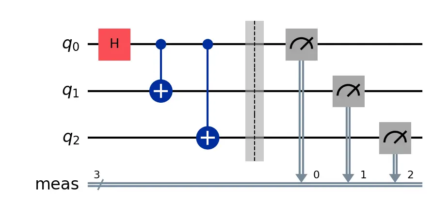
Figure 1: Quantum circuit for constructing the three-qubit Greenberger-Horne-Zeilinger state.
In an ideal case both $\ket{000}$ and $\ket{111}$ would be observed with a $50\%$ probability and no other states should be observed. However, due to errors and noise, states other than $\ket{000}$ or $\ket{111}$, such as $\ket{010}$ or $\ket{110}$, may also be observed. Nevertheless, the states $\ket{000}$ and $\ket{111}$ should be the most common states observed and the other measurement outcomes should be a clear minority even on current-day quantum computers. Fig. 2 shows a histogram of the raw counts obtained directly from VTT Q50 without any error mitigation, and the counts after readout error mitigation has been applied to them.
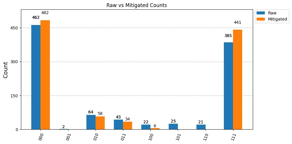
Figure 2: A histogram of raw and mitigated counts.
| 000 | 001 | 010 | 011 | 100 | 101 | 110 | 111 | |
|---|---|---|---|---|---|---|---|---|
| Raw | 462 | 2 | 64 | 43 | 22 | 25 | 21 | 385 |
| Mitigated | 482 | 0 | 58 | 34 | 6 | 0 | 0 | 441 |
| Change | +20 | -2 | -6 | -9 | -16 | -25 | -21 | +56 |
Table 1: Raw and mitigated counts of result states.
As can also be seen from Fig. 2 and Table 1, adding readout error mitigation to the raw counts significantly reduces the frequency of the erroneous measurement outcomes and increases the frequency of the ideal measurement outcomes. Before readout error mitigation, $17.3\%$ of the obtained counts were erroneous. After readout error mitigation, this drops to $9.6\%$.
It should be noted that the quantum job was executed with shots=1024 and hence the raw counts sum to 1024. However, the mitigated counts sum to 1021. The reason behind this is that M3 returns a quasi-probability distribution and not counts. As quasi-probability distributions may have negative values, the distribution is mapped to the nearest probability distribution before the counts can be obtained. This process may cause the number of mitigated and raw counts to differ slightly.
Code
The code used for the example can be found below. First the Qiskit code and then the bash script for submitting the job. For your own experiments it is strongly encouraged to see the EMS documentation for all available features.
Automatic
import os

from iqm.qiskit_iqm import IQMProvider
from qiskit import QuantumCircuit, transpile
from qiskit.visualization import plot_histogram

from fiqci.ems import FiQCIBackend

def ghz_circuit(num_qubits):
    '''
    Construct a quantum circuit that prepares an n-qubit GHZ state.

    Args:
        num_qubits (int): Number of qubits in the GHZ state

    Returns:
        circuit (QuantumCircuit): A quantum circuit
    '''

    circuit = QuantumCircuit(num_qubits)
    circuit.h(0)
    for i in range(1, num_qubits):
        circuit.cx(0, i)
    circuit.measure_all()

    return circuit

# Accessing Q50
Q50_CORTEX_URL = os.getenv('Q50_CORTEX_URL')
provider_q50 = IQMProvider(Q50_CORTEX_URL, quantum_computer="q50")
backend_q50 = provider_q50.get_backend()
# Set up the mitigated backend
# Mitigation levels 0–3 are defined
# Mitigation level 0: no error mitigation applied
# Mitigation level 1: adds readout error mitigation
# Mitigation level 2: adds dynamical decoupling on top of level 1
# Mitigation level 3: adds Pauli twirling on top of level 2
mitigated_backend_q50 = FiQCIBackend(backend_q50, mitigation_level=1, calibration_shots=2048, calibration_file="cals.json")

# Create the circuit
qc = ghz_circuit(3)
# Transpile for specific qubits
qubits = ["QB9", "QB3", "QB8"]
qubit_indices = [backend_q50.qubit_name_to_index(q) for q in qubits]
qc_transpiled = transpile(qc, backend=backend_q50, initial_layout=qubit_indices)

# Run the circuit on the backend with error mitigation
shots = 1024
job = mitigated_backend_q50.run(qc_transpiled, shots=shots)
mitigated_counts = job.result().get_counts()
print(f'Counts with error mitigation: {mitigated_counts}')

# For comparing the results, also get the raw counts
raw_counts = job.result().results[0].header["fiqci_ems"]["raw_counts"]
print(f'Counts without error mitigation: {raw_counts}')
Manual
import os

from iqm.qiskit_iqm import IQMProvider
from qiskit import QuantumCircuit, transpile
from qiskit.visualization import plot_histogram
from fiqci.ems.mitigators.rem import M3IQM
from fiqci.ems.utils import probabilities_to_counts

def ghz_circuit(num_qubits):
    '''
    Construct a quantum circuit that prepares an n-qubit GHZ state.

    Args:
        num_qubits (int): Number of qubits in the GHZ state

    Returns:
        circuit (QuantumCircuit): A quantum circuit
    '''

    circuit = QuantumCircuit(num_qubits)
    circuit.h(0)
    for i in range(1, num_qubits):
        circuit.cx(0, i)
    circuit.measure_all()

    return circuit

# Accessing Q50
Q50_CORTEX_URL = os.getenv('Q50_CORTEX_URL')
provider_q50 = IQMProvider(Q50_CORTEX_URL, quantum_computer="q50")
backend_q50 = provider_q50.get_backend()

# Create the circuit
qc = ghz_circuit(3)
# Transpile the circuit for specific qubits
# If you wish to use different physical qubits, change the qubit names here to match the qubits you wish to use
qubits = ["QB9", "QB3", "QB8"]
qubit_indices = [backend_q50.qubit_name_to_index(q) for q in qubits]
qc_transpiled = transpile(circuits=qc, backend=backend_q50, initial_layout=qubit_indices)
# Define the number of shots
shots = 1024
# Get counts with no mitigation
raw_counts = backend_q50.run(qc_transpiled, shots=shots).result().get_counts()
print(f'Counts without error mitigation: {raw_counts}')

# Initialize mitigator
mitigator = M3IQM(backend_q50)
# Calibrate for specific qubits
mitigator.cals_from_system(qubits=qubit_indices, shots=2048, method="balanced", cals_file="cals.json")
# Apply readout error mitigation
quasi_dist = mitigator.apply_correction(raw_counts, qubits=qubit_indices)

# Get the nearest probability distribution
mitigated_dist = quasi_dist.nearest_probability_distribution()
# Get mitigated counts
mitigated_counts = probabilities_to_counts(mitigated_dist, shots)
print(f'Counts with error mitigation: {mitigated_counts}')
Bash
FiQCI EMS is included in the fiqci-vtt-qiskit module, so using FiQCI EMS does not require any changes to the example batch script provided in the CSC docs.
#!/bin/bash -l

#SBATCH --job-name=ems_quantumjob   # Job name
#SBATCH --output=ems_quantumjob.o%j # Name of stdout output file
#SBATCH --error=ems_quantumjob.e%j  # Name of stderr error file
#SBATCH --partition=q_fiqci   # Partition (queue) name
#SBATCH --ntasks=1              # One task (process)
#SBATCH --mem-per-cpu=2G       # memory allocation
#SBATCH --cpus-per-task=1     # Number of cores (threads)
#SBATCH --time=00:05:00         # Run time (hh:mm:ss)
#SBATCH --account=project_xxx  # Project for billing

module use /appl/local/quantum/modulefiles
module load fiqci-vtt-qiskit

export DEVICES=("Q50")

source $RUN_SETUP

python -u ems_quantum_job.py
Conclusion
In summary, error mitigation provides a straight-forward way to improve the quality of results on current NISQ hardware. The FiQCI error mitigation service offers the ability to incorporate error mitigation into users’ existing workflows running on LUMI. Already a simple readout error mitigation reduces erroneous outcomes and brings the measured distributions closer to ideal results.
It should be noted that readout error mitigation is most effective when readout errors are the dominant source of noise. If gate errors are significant, REM alone will not bring results close to the ideal distribution. For circuits with high gate error rates or significant decoherence, other mitigation techniques such as zero-noise extrapolation will be needed alongside REM to see meaningful improvement. More advanced features will be added soon!
References
- Cai, Z., Babbush, R., Benjamin, S. C., Endo, S., Huggins, W. J., Li, Y., McClean, J. R., & O’Brien, T. E., “Quantum error mitigation”, Reviews of Modern Physics, 95(4), 045005, 2023. doi: https://doi.org/10.1103/RevModPhys.95.045005
- Nation, P. D., Kang, H., Sundaresan, N., & Gambetta, J. M., “Scalable Mitigation of Measurement Errors on Quantum Computers”, PRX Quantum, 2, 040326, 2021. doi: https://doi.org/10.1103/PRXQuantum.2.040326
- https://qiskit-community.github.io/qiskit-experiments/manuals/measurement/readout_mitigation.html [Accessed: Jan. 12 2026]
- https://www.ibm.com/quantum/blog/mthree-qiskit-extension [Accessed: Jan. 12 2026]
- https://qiskit.github.io/qiskit-addon-mthree/ [Accessed: Jun. 3 2026]
- https://github.com/Qiskit/qiskit-addon-mthree/blob/main/mthree/iterative.py [Accessed: Jan. 12 2026]
Additional Resources
- Additional information about Mthree is available in this blog.
- Qiskit’s Mthree documentation
- FiQCI error mitigation service GitHub repository
- FiQCI EMS Documentation